
So if you read the title of this blog and decided to click on it anyway I applaud you fellow nerd. I hope you will find this as interesting as I did while creating it. Recently I watch Veritasium’s video (linked below) explaining the how, what and why of a brachistochrone and the history of how it was conceived of. Ok, I lost most of you already, so lets take a step back shall we.
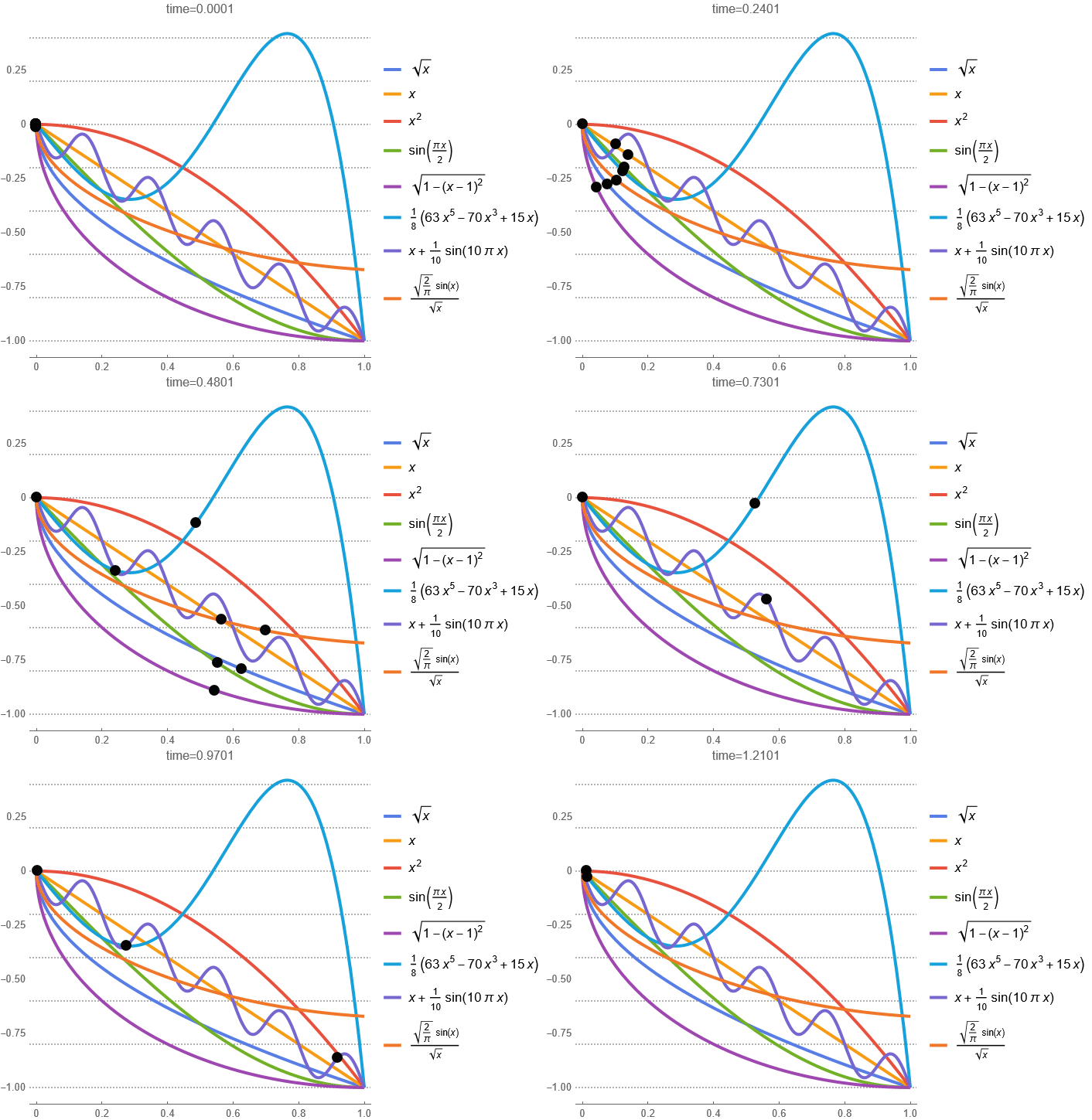
/brəˈkɪstəkrəʊn/
The brachistochrone problem is a famous question in physics and calculus that asks: What is the fastest path that an object should take to move between two points under the force of gravity? Specifically, it seeks the curve that will allow an object to slide (without friction) from one point to another in the shortest possible time, under the influence of gravity alone.
At first, you might think that the straight-line path between the two points is the quickest route but surprisingly, it’s not! The fastest path is actually a special type of curve called a cycloid. This is the same curve traced by a point on the rim of a rolling wheel, like if you put a dot of paint on a bicycle tire and watched it move as the wheel rolled forward.
To understand why a straight line isn’t the fastest route, think of the brachistochrone problem like a race track. If you’re sliding down a hill, you want to pick up as much speed as possible. The cycloid shape dips down quickly at first, allowing the object to gain speed quickly, and then gradually levels out as it approaches the destination. This combination allows the object to reach the endpoint faster than if it took a straight line or a different curved path.
To break it down a bit more:
The Problem: You have two points one higher up and one lower down and you want to find out what path will get a ball from the top point to the bottom in the shortest time.
The Intuition: It might seem that a straight line is the fastest, because it is the shortest distance. But that doesn’t take advantage of gravity in the most efficient way to gain speed.
The Solution: The brachistochrone curve, which is a cycloid, allows the object to initially gain speed very quickly because it descends steeply. Then, it transitions into a shallower slope to maintain that speed effectively. This path minimizes travel time.
This problem was originally posed by the mathematician Johann Bernoulli in 1696, and it was a big moment in the history of physics and calculus because it helped illustrate the power of optimization methods and calculus of variations. The solution also involves interesting physics concepts like gravitational acceleration and conservation of energy.
The brachistochrone problem shows how nature is often counterintuitive sometimes the shortest distance isn’t the fastest route. Instead, it’s the one that allows the right balance of speed and direction, which is what makes the cycloid the winning shape.
Right now that we are caught up a little bit more lets get to my proof of concept experiment. So I will be the first to admit when saw all those mathematical symbols in the video my my mind went to a sun baked beach while listening to the waves breaking on the rocks.
However, after returning to reality, I started thinking. It was nice to learn about how mathematicians, both past and present, derived the formulas for the brachistochrone. But I wondered if there might be another way. Then I thought to myself, “Hey, I know a bit about genetic algorithms and coding. What if I created a GA to try to find the best curve to minimize the time it would take for a ball to roll from point A to point B?” And that’s where the rabbit hole opened, with an anxious white rabbit saying, “Why not try it?” along with, “You might be late,” even though I was doing all of this in my spare time. Before I dive into the journey, let’s take another quick detour so you can follow along later.
What is a genetic algorithm?
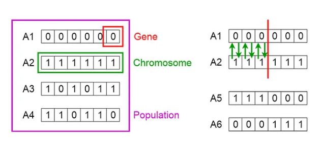
In short a genetic algorithm (GA) is a type of computer algorithm inspired by the process of natural selection. It’s used to solve problems by mimicking the way evolution works in nature. Here’s a simple way to think about it:
Imagine you’re trying to solve a puzzle but don’t know the solution in advance. A genetic algorithm starts by creating a “population” of random solutions to the puzzle. These solutions aren’t great at first; they’re kind of like rough guesses. Each “solution” is like a “creature” that has certain “traits” (in this case, features that represent parts of the solution).
Here’s how it works step by step:
Initialization: The algorithm creates a set of random solutions (the population).
Selection: It then evaluates each solution, scoring them based on how close they are to the desired outcome. The best-performing solutions are more likely to be “selected” to create the next generation.
Crossover (Recombination): The algorithm combines parts of two good solutions to create new ones, hoping these combinations will be even better. This is like “mating” two creatures to produce offspring with mixed traits.
Mutation: Sometimes, a small random change is made to some solutions. This introduces variety and helps the algorithm explore different possibilities, similar to genetic mutations in nature.
Iteration: The process repeats over many generations. With each new generation, the solutions get closer and closer to the ideal answer.
Over time, through selection, crossover, and mutation, the algorithm evolves solutions that are better at solving the puzzle. Eventually, it finds a solution that’s good enough for the problem it’s trying to solve. In essence, a genetic algorithm is a way for a computer to learn the best solution to a problem by simulating evolution. It’s commonly used in optimization problems where finding the exact solution is difficult or time-consuming.
Here is some links to some useful videos if you want to know even more.
Computerphile
Steve Brunton
DigitalSreeni
Now that we’re all caught up on the theory, let’s get to the fun part, shall we? These days, saying you used an LLM or AI to help you code is like admitting you’re using a knife and fork at the dinner table. However, it’s still very much a partnership. Trying to instruct and code an LLM to create a complex project all in one go is like handing a toddler a one-page list of bullet points to follow until they graduate—and then getting upset when the toddler can’t even get to school on time. So, baby steps.
First, I set out to create the physics engine. You’d think, with all the millions of Python libraries out there, there’d be one that just works, right? Nope. I spent more time than I’d like to admit getting a half-decent, realistic physics engine up and running. I also had to tweak things like friction, since this experiment requires little to no friction to work. But in the end, I got a simulation that would not only let a ball drop but would also allow it to collide with objects.
I decided to use Pygame, which I’ve used in some other projects that you might see in future blogs. Pygame is useful because it handles most of the complex physics and also has GPU acceleration built in, so you can run your applications at really high frame rates. This is perfect for me, as I can speed up time and run simulations much faster than real-time speed. Pretty cool, if I do say so myself! My Nobel Prize has been sent via the SA post office, so I’m still waiting for it to be delivered.
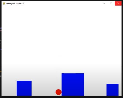
Next, after setting up the physics and getting the ball to collide with a single block, I decided to add more blocks to see if the ball would roll down a hill. This is where I had to adjust the friction, as initially, it was like tossing a sticky ball against a wall and watching it slowly crawl down. (I’m sure we all had those toys growing up, so you know what I’m talking about!) But in the end, I managed to get a ball that would roll well, more like bounce, due to the size of the steps but it worked.
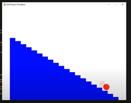
I added more blocks, making the ramp a bit smoother, and I also included a “stopper” at the end. This stopper not only stopped the ball but also served as the “end goal” to stop the timer, allowing me to measure how long it took the ball to travel from point A to point B. So far, so good! I also saved the height of each block into a list for easier access later on.
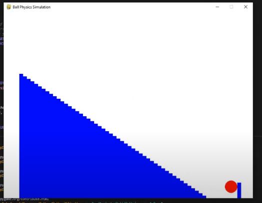
Since I’d already added more blocks, I thought, why not add so many that you can’t even see them anymore, creating what looks like a smooth ramp? However, I realized that continuously adding more blocks to smooth out the ramp wasn’t sustainable. The platform the ball was rolling on was getting increasingly complex, especially since I wanted to save the height of each bar for every member in the population. Even without testing, I knew this would lead to a very slow simulation.
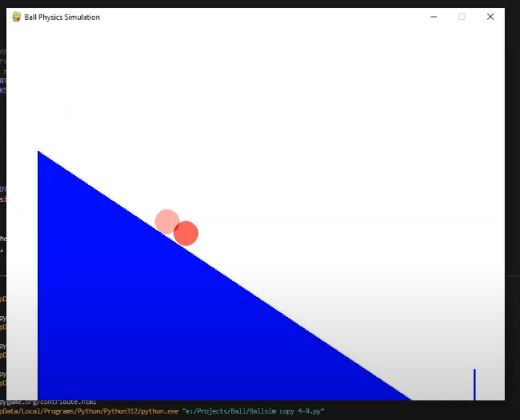
I had a nice ramp, but I wanted to extend it a bit to give the ball more room to roll. So, I adjusted the size of the simulation window, as the width of the bars was linked to the window’s X dimension. Now we were getting somewhere. And yes… for each step, I ran the simulation many, many times. Watching a virtual ball roll down a virtual hill never gets old.
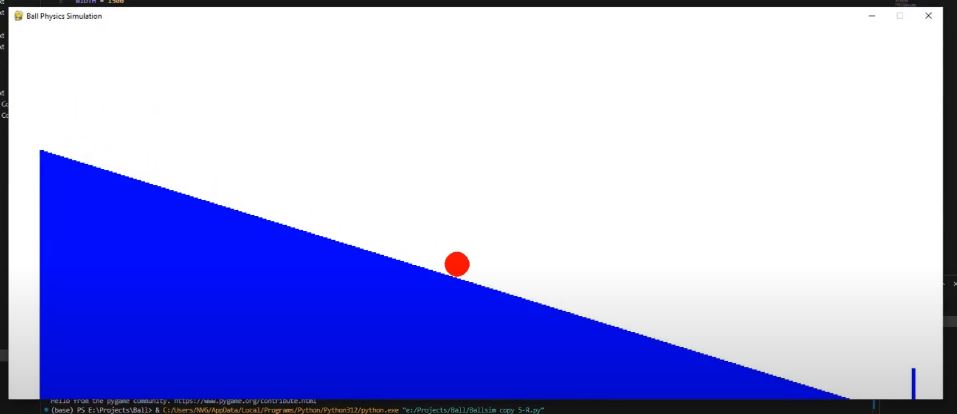
Now came the next fun part: adding the genetic algorithm into the mix. See? I told you reading all the information above would help! I created a population of 200 and planned for the top 50 members of each generation to advance to the next. Well, that was the idea, at least. With the current setup, I initialized the height of each bar randomly and let only the best ones move onto the next cycle. The issue was that, because the hill was so “spiky” (official term I’m using now), the ball never really traveled very far, leaving the “best” of each population still mostly random.
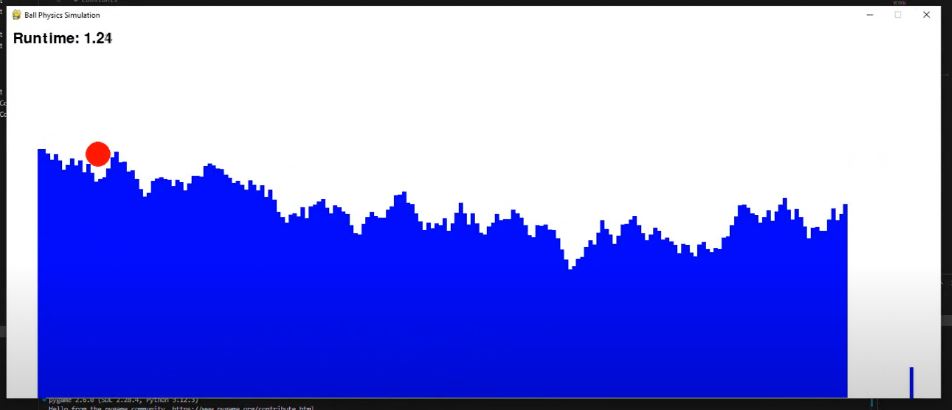
I then decided to add a smoothing step to the current layout of the bars to even out the very high or low bars that were stopping the ball from making progress. I also added a metric to track how far the ball traveled for each member in the population. This metric would then serve as the fitness function, helping determine which members would pass their genes onto the next generation.
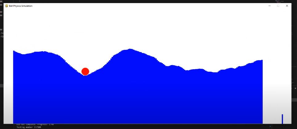
Most of the time, this approach worked fine, however, there were too many instances where the ball would bounce or get stuck on a small “ridge” caused by a block positioned just a little too far from its neighbor. To solve this, I replaced the blocks with a single polygon. By setting a base for the polygon and using the height as the Y-coordinate of the top edge, I could create a smooth, continuous surface. This change eliminated the bumps from the individual blocks, resulting in a super-smooth hill the ball could roll on as much as it pleased.
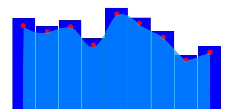
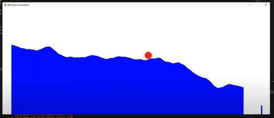
I noticed that, because the heights of the blocks were random, the beginning and end of the (hopefully soon-to-be) ramp didn’t stay fixed. I solved this by locking down the first and last bars at the minimum and maximum heights, respectively. This initially led to awkward, sharp lines between the start/end blocks and their neighbors. To smooth out these differences, I added a “fade in” effect, which helped transition smoothly when there was a significant height difference between the fixed blocks and the next blocks. The result was a nice transition from the locked blocks to the others, which were free to vary wildly in height.
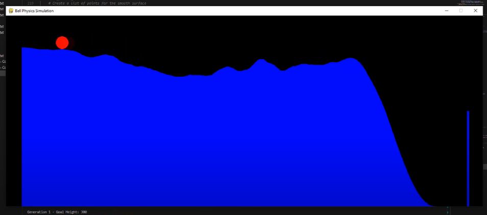
And there you have it! Below is a video showing all the steps in action, as I think this conveys the process much better than just seeing screenshots.
Now, it’s time to show off the final product and see if my theoretical approach actually translates to practical results. The video below captures a few minutes from the start of the process. Working with AI, I have to resist calling this “training,” as I see this simple process more as an iterative selection loop that picks the best outcome repeatedly. Then again, that’s essentially what most modern AI algorithms do but let’s not dive into a philosophical debate.
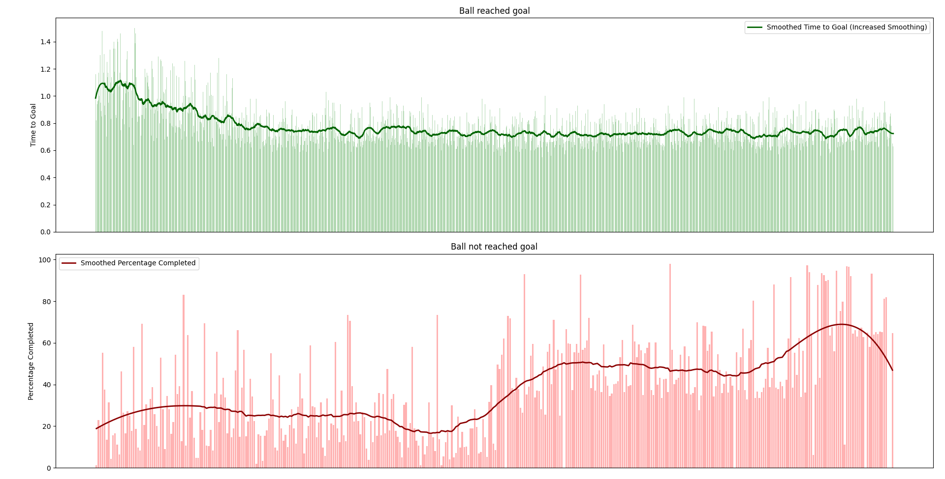
You’ll notice that the text displayed in the terminal is either red or green. If the text is red, it means the ball didn’t reach the end, and only the distance traveled along the X-axis was recorded as a percentage of progress. The closer the ball got to the goal, the higher the progress percentage.
If the text is green, it means the ball reached the goal, and in this case, the time taken from start to finish was recorded. When no member of the population managed to get the ball to the goal, those with the highest progress were selected to advance to the next round. If any member did get the ball to the end, they took priority in selection, with secondary scoring based on the quickest time.
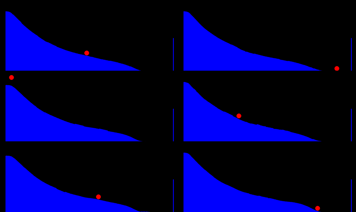
Below is a quick time-lapse I created. I added a few lines of code to take a screenshot of the window and save it in a separate folder before each run. At the beginning, you’ll see almost pure randomness, but very quickly, it falls into an “almost” ideal pattern. If you watch the whole clip (I recommend 2x speed), you’ll notice the “bump” at the bottom of the ramp gradually shrinking, as having a bump near the end slows the ball down.
Keep in mind, this time-lapse only covers the first hour or so. The final ramp was the result of running the evolution overnight, but to avoid managing millions of screenshots, this clip only shows the initial phase. It still provides a solid glimpse into what’s happening in the background.
Below is a quick graph I created based on the time-lapse above. The red graph represents only the first few populations, as the genetic algorithm quickly develops ramps where the ball consistently reaches the end. The green graph spans a longer timescale, showing that the algorithm soon stabilizes around an average completion time of approximately 0.7 seconds.
And finally, below are the results of all this experimentation. You can see that the ramp has evolved into a shape that seems to optimize the ball’s time to reach the goal. Just for fun, I decided to overlay an actual brachistochrone curve on the ramp to see how close the genetic algorithm got. If you squint and tilt your head a bit, you can see the resemblance between the evolved ramp and the brachistochrone shape. I’m confident that if I let the evolution run even longer, the little bump at the end would have smoothed out as well.
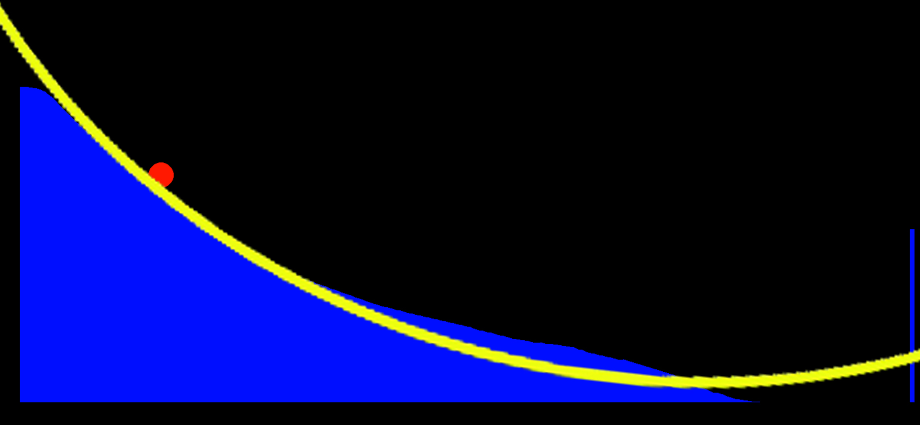
Please keep in mind that this was just an experiment to test if my theory could actually yield any results. I’m fairly certain this has no practical application, but it’s still exciting to see that an algorithm like the genetic algorithm used here can generate a rough approximation of something typically derived through pure mathematics. So, I’d say this little side project was a success! I’ll reward myself with a pizza for all my hard work and perhaps extend a kind “Thank you” to all the LLMs that helped speed up the project.
If you’re interested in learning more about the brachistochrone, here are a few videos, including the one that started me down this rabbit hole.

