

Ever since I went behind the curtain of AI, I have been fascinated by how AI can learn almost anything. Sure, seeing the result of a good linear regression is impressive, but seeing, say, an AI learn to drive a 2D car around a track is truly fascinating to me. This, to me, is the core of AI. Yes, I know there are a ton of AI uses and algorithms, but I find reinforcement learning to be a particularly interesting subfield of AI in general.
Below is my account of my journey to understand this specific field of machine learning. I spent the last four or five months getting to grips with the very basics of reinforcement learning, and below is a summary of my learning path. I now have even more respect for those who had to learn without the aid of AI to answer even the most mundane questions repeatedly.
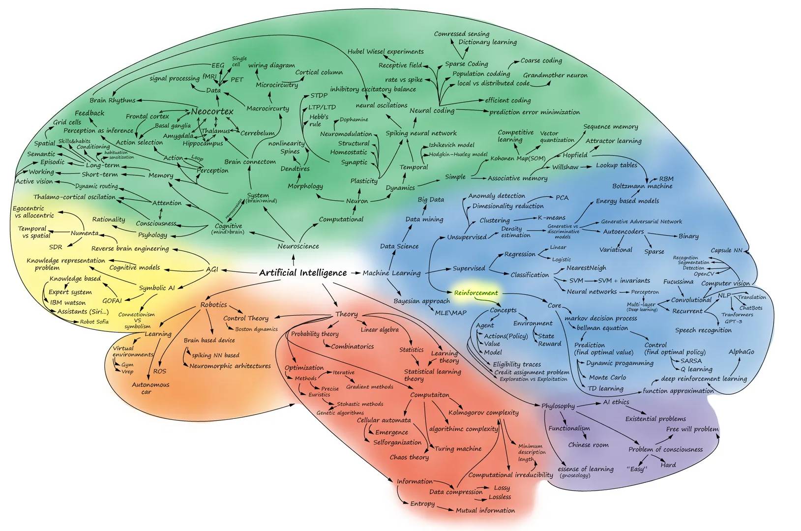
So, I decided to take on a bit of a harder challenge and do a deep dive into the world of reinforcement learning. Something that I see is the next step following generic algorithms. This below is my journey in getting to know a little bit more about what is going on under the hood of RL.
What is reinforcement learning?
But first, what is reinforcement learning? Is it something that will aid the AI overlords to control android bodies and enslave all of humanity? Perhaps, but let’s stay positive, shall we, and use the tools we have for our benefit in the meantime.
Reinforcement learning (RL) is a branch of artificial intelligence (AI) focused on training agents to make a sequence of decisions within an environment in order to achieve a specific goal or maximize some notion of cumulative reward. Unlike supervised learning, which relies on labeled examples, or unsupervised learning, which looks for hidden patterns in unlabeled data, reinforcement learning draws inspiration from the way humans and animals learn through trial and error. An RL agent explores its environment, takes actions, receives feedback in the form of rewards or penalties, and gradually refines its strategy to improve future outcomes.
Within the broader AI landscape, reinforcement learning sits at the intersection of machine learning, decision theory, and optimization. While supervised and unsupervised techniques excel at recognizing patterns or extracting insights from static datasets, reinforcement learning shines when dealing with dynamic, interactive scenarios. For example, it’s well-suited for teaching autonomous vehicles to navigate safely, helping industrial robots refine their assembly techniques, enabling game-playing agents like AlphaGo to strategize moves, or even managing inventory in a supply chain. In essence, RL plays a pivotal role when the goal is not just to learn from data, but to learn how to act in an environment in pursuit of long-term objectives.
Looking at a very NEAT Actor-Critic RL’s
I’ve decided to look at two types of RL. First, an older and more classic version called NEAT, and then a look at a more modern version called Actor-Critic RL. You have to know where it all began if you want to progress and learn anything new. So, I decided to start with the basics and work from there. Since NEAT uses genetic algorithms as its basis, I thought I would include this in my study as I’m rather familiar with how GEs work. But what is the difference between the two? Here is a short description of each. Later, I will do a bit more in-depth explanation of each.
NEAT (Neuro Evolution of Augmenting Topologies):
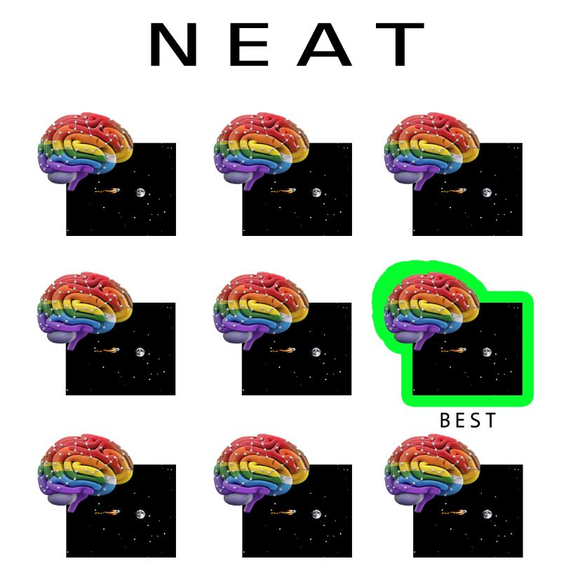
NEAT (Neuro Evolution of Augmenting Topologies):
NEAT is an evolutionary approach to reinforcement learning that evolves both the structure and weights of neural networks over time. Instead of starting with a fixed network architecture, NEAT begins with simple neural networks and incrementally grows their complexity by adding new neurons and connections through genetic mutations. This allows it to discover not only an effective set of parameters, but also an efficient network topology that is well-suited for the given task. The process involves a population of candidate solutions (neural networks), each scored according to its performance in the environment. The best-performing networks are then allowed to “reproduce” with mutation and crossover operations, creating a new generation with slightly varied architectures. Through many generations, NEAT refines both the structure and parameters of the networks, potentially uncovering novel and highly specialized architectures that can achieve strong performance without requiring human-designed network structures.
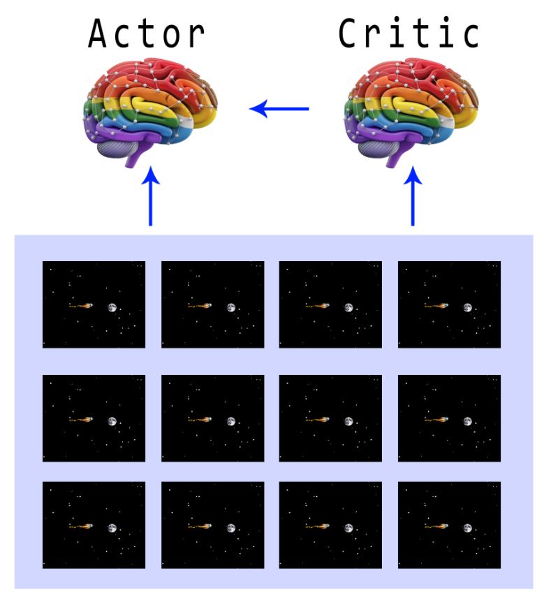
Actor-critic methods are a class of reinforcement learning algorithms that combine the strengths of two key ideas: the actor and the critic. The “actor” is responsible for selecting actions, essentially learning a policy that maps states of the environment to actions. The “critic,” on the other hand, evaluates how good the chosen actions are by estimating a value function, essentially predicting future returns. By working together, these two components create a feedback loop where the actor updates its behavior based on the critic’s assessment, while the critic refines its estimates based on the outcomes it observes. This approach elegantly balances exploration and exploitation, often converging more smoothly and efficiently than methods that rely solely on policy gradients or value-based updates. Actor-critic methods have formed the basis for a variety of successful RL algorithms, including SAC and PPO, which are widely used in complex tasks such as robotics, game playing, and continuous control tasks.
In case you were wondering, in Reinforcement Learning (RL), the concepts of exploration and exploitation guide how an agent learns to choose actions:
- Exploration: The agent tries actions it hasn’t taken often or at all, even if they are not currently known to yield high rewards. This helps the agent gather new information about the environment, learn from mistakes, and potentially discover better strategies over time.
- Exploitation: The agent leverages its existing knowledge about which actions are most rewarding and repeatedly chooses them to maximize its expected return. This can ensure a high immediate payoff but may prevent the agent from uncovering even more valuable actions it has yet to try.
In RL, balancing exploration and exploitation is a key challenge. Too much exploration means slow learning and delayed gains, while too much exploitation can lead the agent to settle for suboptimal solutions. Effective RL methods include mechanisms, such as epsilon-greedy policies, upper confidence bounds, or entropy regularization, to maintain an appropriate balance between these two approaches.
Although both NEAT and Actor-Critic methods can leverage multiple game instances, they do so in fundamentally different ways. In a NEAT-based setup, each game instance is typically played by a unique neural network taken from a population, allowing the evolutionary algorithm to evaluate many candidate architectures and parameters simultaneously. This means there is a large, diverse set of neural networks running in parallel, each trying out different strategies. In contrast, actor-critic methods generally maintain a single actor network and a single critic network, even when multiple environments are run in parallel. In this scenario, the multiple game simulations provide a richer stream of experiences for just these two networks, which share and aggregate the learning signals to improve their joint policy-value estimates. Thus, while NEAT spreads its exploration across a variety of evolving architectures, actor-critic methods direct parallelization toward collecting more varied experiences for a single, ongoing policy.
What is NEAT precisely?
NEAT (NeuroEvolution of Augmenting Topologies) is an approach to creating and improving artificial neural networks using ideas from evolution. In simple terms, NEAT doesn’t just adjust the “weights” of a fixed neural network like many traditional methods do, it also tries to build better and more complex networks from scratch, step by step, through a process similar to natural selection using generic algorithms.
Here’s the main idea of how it works:
- Start with simple networks: At the beginning, NEAT creates a bunch of very simple neural networks. Each one might only have a few neurons and connections. Think of these as “creatures” in a population.
- Test each network’s performance: Each network is given a problem to solve (for example, guiding a virtual robot through a maze). We measure how well it performs—this is often called its “fitness score.”
- Select the best networks: The networks that perform better are more likely to have “offspring.” This means the best solutions move on to the next generation, just like animals that are better adapted to their environment are more likely to reproduce.
- Introduce variations (mutations) to grow complexity: When creating the next generation of networks, NEAT doesn’t just tweak the connection weights (the numbers that determine how strongly neurons talk to each other). It can also add new neurons or new connections between neurons. This is like evolving a new type of “brain wiring” over time. The idea is that, across many generations, the networks will become more sophisticated and better at solving the problem.
- Speciation to protect innovation: NEAT also uses a concept called “speciation.” It groups networks into species based on how different their connections and structures are. This prevents new, unusual network structures from being immediately wiped out by competition with well-adapted but simpler networks. By grouping similar networks together, NEAT gives these new ideas some breathing room to develop and improve.
After running through many generations of this evolutionary process, the result is often a highly effective neural network—one that has “grown” its own architecture to handle the problem at hand, rather than relying on a human-designed structure.
To summarize, NEAT is like an evolutionary breeding program for neural networks. It starts simple, picks out the best performers, and gradually encourages new and more complex “brains” to form, hoping that, over time, these evolving neural networks will discover better ways to solve the given problem.
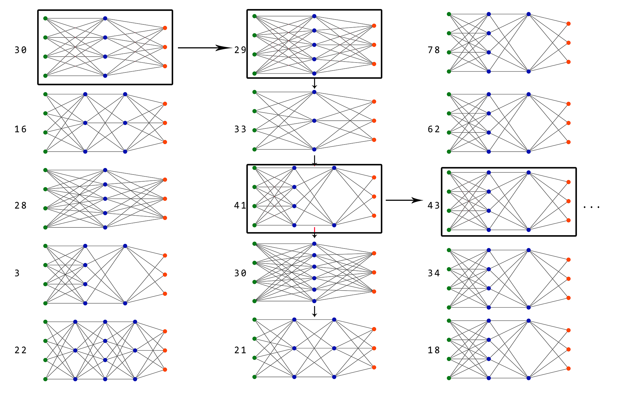
Below is a rough representation of how a neural network would evolve using the NEAT algorithm. Each generation would then represent the best network being carried over to the next.
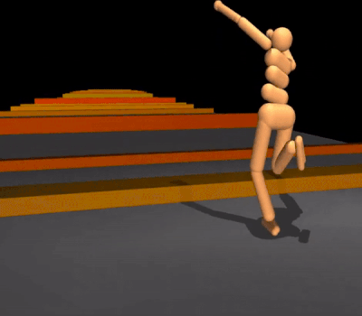
So now it’s time to put all this theory to the test. Not knowing really where to start, I did not want to start with trying to break new ground in the world of RL, but rather just get to grips with how things work and see if I can actually build something that is trainable. This is why I decided to copy the “Dino game” you see when you do not have internet. And for those who did not know, if you press the “UP” key on your keyboard, you can actually play a game and it’s not just a simple “dumb” image when there is no internet.

Yes, you heard it here first, kids: the image you see when there is no internet is an actual game. And I’ve spent way too much time on this, even sometimes disabling my Wi-Fi just to play it. You know, for science.

However, I did not want to spend additional time creating a “link” to the actual Dino game in your browser, along with the inputs and outputs you would need to train an AI to play the game. So, I decided to just create a very simple version of it myself for the AI to train with. I again used Pygame as the base, as this one seems to get the best results in building real-time games in Python.
The game itself is really simple: the AI can duck, jump, or do nothing. Thinking back, I probably could have left out the “do nothing” part, but oh well – it worked. And the rule of programming is not to fix something that is not broken. I added obstacles for the AI to either jump over or duck under. Fun note: in the beginning, I made the red obstacles not high enough, and the AI just kept on jumping over everything. I also added a graph on the top right to show the fitness of every population. Basically, the best distance any member of the specific population traveled. I found a nice number of about 100 members per population was sufficient to get good training times. I could have made it 1,000 members in the population, and then it would most of the time “get lucky” even in the first generation, but where’s the fun in that?
I will admit that learning what each part of the config file for the NEAT algorithm does took me a while, as I had to fine-tune each parameter bit by bit until I got a setup where the model was training quickly and giving good results. Below is an explanation of each setting in the NEAT config file:
fitness_criterion = max: NEAT often runs a population of genomes and calculates a fitness value for each. The fitness_criterion determines how the “winner” or the top-performing genomes are selected at each generation. Here, max means the fitness values are compared and the best (highest fitness) individuals in the population or species are considered leaders. This is the typical approach to selecting top genomes.
fitness_threshold = 2000:This sets a stopping condition for the evolutionary run. If any genome in the population reaches or exceeds a fitness score of 2000, the evolution can be terminated early. In other words, if you’ve defined a certain fitness as “solving” the problem, you can stop once it’s achieved.
pop_size: This sets the size of the population of genomes in each generation.{POPULATION_SIZE} is a placeholder to be replaced by a chosen number. For example, if pop_size = 100, each generation will have 100 genomes to evaluate.
reset_on_extinction: If True, when all species go extinct (no individuals survive, or no species meet reproduction criteria), the population is reset from scratch (e.g., starting over with a new initial population). If False, no automatic reset occurs on extinction, which may just end the run if no population remains.
Default Genome Section:
The DefaultGenome section specifies how individual neural network genomes are initialized and mutated. Each genome corresponds to one neural network architecture and its parameters.
Node activation options:
- activation_default = sigmoid Each node’s activation function transforms the sum of its weighted inputs into an output. The default activation here is the
sigmoidfunction. - activation_mutate_rate = 0.0 This is the rate at which a node’s activation function may be changed during mutation. With 0.0, the activation function will never change from its default.
- activation_options = sigmoid This lists all possible activation functions the node can mutate to if
activation_mutate_rate> 0. Here, onlysigmoidis allowed, so even if mutation was enabled, it would have no effect.
Node aggregation options
- aggregation_default = sum. Each node combines its inputs using an aggregation function (e.g., sum, product, max). The default here is a simple summation of inputs.
- aggregation_mutate_rate = 0.0. Similar to the activation function, this sets how often the aggregation function might mutate. With 0.0, it never changes.
- aggregation_options = sum. Available aggregation functions are listed here. Since it’s only
sum, no changes to aggregation are possible.
Node bias options
- bias_init_mean = 0.0 and bias_init_stdev = 1.0. When a new node (or genome) is initialized, its bias is chosen from a distribution with a mean of 0.0 and a standard deviation of 1.0, typically a normal distribution.
- bias_max_value = 30.0 and bias_min_value = -30.0. This clamps the bias so that it can’t evolve beyond these bounds. Keeps biases within a reasonable range.
- bias_mutate_power = 0.5. When a bias mutates, its new value is chosen by adding a random value drawn from a distribution with a standard deviation of
bias_mutate_powerto the current bias. Essentially controls the “step size” of bias mutations. - bias_mutate_rate = 0.7. This is the probability that a node’s bias will undergo a mutation in a given generation. High (0.7) means bias mutation is relatively common.
- bias_replace_rate = 0.1. This is the probability that instead of perturbing the bias by adding a small value, the bias is replaced entirely with a new random value drawn from the initial distribution.
Node response options
- response_init_mean = 1.0 and response_init_stdev = 0.0. The “response” parameter (less commonly used in some NEAT variants) can scale the output of a node. A
stdevof 0.0 means the initial response is always 1.0. - response_max_value = 30.0 and response_min_value = -30.0. Similar to bias, it constrains the range of the response parameter.
- response_mutate_power = 0.0. Indicates that no perturbation occurs (if mutation were allowed).
- response_mutate_rate = 0.0 and response_replace_rate = 0.0. No mutations occur to the response parameter at all. This essentially disables response parameter mutation.
Genome compatibility options
- compatibility_disjoint_coefficient = 1.0 and compatibility_weight_coefficient = 0.5
In NEAT, the genetic distance between two genomes is calculated based on:- Disjoint and Excess Genes: Genes that don’t match between two genomes.
- Matching Genes’ Weight Differences: The average difference in connection weights for matching genes.
The genetic distance is something like:
distance = (c1 * (#disjoint_genes / N)) + (c2 * (#excess_genes / N)) + (c3 * average_weight_diff)
Here,compatibility_disjoint_coefficientlikely corresponds toc1andcompatibility_weight_coefficienttoc3(assumingc2is the same asc1or also defined, depending on the exact code). These coefficients control how strongly differences in topology and weights affect species separation.
Connection add/remove rates
- conn_add_prob = 0.5. The probability of adding a new connection (edge) between two unconnected nodes during mutation. This encourages more complex topologies over time.
- conn_delete_prob = 0.5. The probability of removing an existing connection during mutation. This can simplify networks that become overly complex.
Connection mutation options
- weight_init_mean = 0.0 and weight_init_stdev = 1.0. When a connection (synapse) is first created, its weight is initialized from a normal distribution with these parameters.
- weight_max_value = 30.0 and weight_min_value = -30.0. The limits for connection weights. Prevents runaway growth of weights.
- weight_mutate_power = 0.5. Similar to bias_mutate_power, this determines the scale of weight perturbations during mutations. A higher value means larger random steps when adjusting weights.
- weight_mutate_rate = 0.8. The probability a connection’s weight will be mutated each generation. 0.8 is quite high, so weights frequently adjust.
- weight_replace_rate = 0.1. The probability that instead of perturbing the weight, the mutation replaces it entirely with a new random value from the initial distribution.
Connection enable options
- enabled_default = True. When a new connection gene is created, it is enabled by default.
- enabled_mutate_rate = 0.01. The probability that an enabled connection may be disabled or a disabled connection may be re-enabled during mutation.
Node add/remove rates
- node_add_prob = 0.2. Probability of adding a new node (via splitting a connection into two nodes) each generation. This is the primary method of increasing network complexity.
- node_delete_prob = 0.2. Probability of removing a node (and associated connections), simplifying the network.
Network parameters
- feed_forward = True. If True, the network is always feed-forward with no recurrent connections allowed. This ensures no cycles form in the connectivity graph.
- initial_connection = full. Determines how the initial population is connected.
fulltypically means every input is connected to every output at the start, ensuring densely connected initial networks. - num_hidden = 0. Starts the networks with zero hidden layers/nodes. Hidden nodes will evolve over time if
node_add_prob> 0. - num_inputs = 4 and num_outputs = 3. Specifies the number of input and output nodes for the evolved networks. The network will receive 4 input signals and produce 3 output signals.
DefaultSpeciesSet:
compatibility_threshold = 3.0. Species are formed by grouping similar genomes together. If the genetic distance (compatibility distance) between a genome and a species’ representative is less than compatibility_threshold, that genome is placed into that species. Lower thresholds lead to fewer species (as they must be very similar), while higher thresholds allow more diversity (more species form).
DefaultStagnation:
species_fitness_func = max. Determines how the fitness of a species is measured to detect stagnation. max means the species’ best genome fitness is used as the representative measure of species performance.
max_stagnation = 20. If a species does not improve (increase in max fitness) for max_stagnation generations, it is considered stagnant. Stagnant species may be removed or reduced in size to make room for more promising lineages.
species_elitism = 2. The number of top-performing individuals in each species that are protected from removal regardless of stagnation or selection. Ensures some genetic material from a species always survives to the next generation, promoting stability and preserving innovations.
DefaultReproduction:
elitism = 2. At the population level, elitism ensures that the top 2 best-performing genomes from the entire population are carried directly into the next generation without modification. This prevents losing the best genome found so far.
survival_threshold = 0.2. After evaluating all genomes in a species, only the top 20% (0.2) of them are allowed to reproduce. The bottom 80% are removed. This encourages improvement over generations by selecting only the top performers to pass on genes.
Below is a video of NEAT learning to play the game in real-time. This has not been sped up and ran on a single CPU. The little “dots” on the left represent the members of each population, all playing at the same time in the same level. This is really survival of the fittest. You will see that most die almost instantly, but there are a few that manage to jump or duck and miss one or two obstacles before also being returned to the land of 1’s and 0’s. The overlaid graph shows the average fitness per population. The idea is for the players to duck under the red pillars and jump over the black ones. You will see that as the neural networks of the populations get better and better, they stay alive for longer and longer. Later, you will even see NEAT splitting populations into species to give them a better chance of becoming the ultimate obstacle champion.
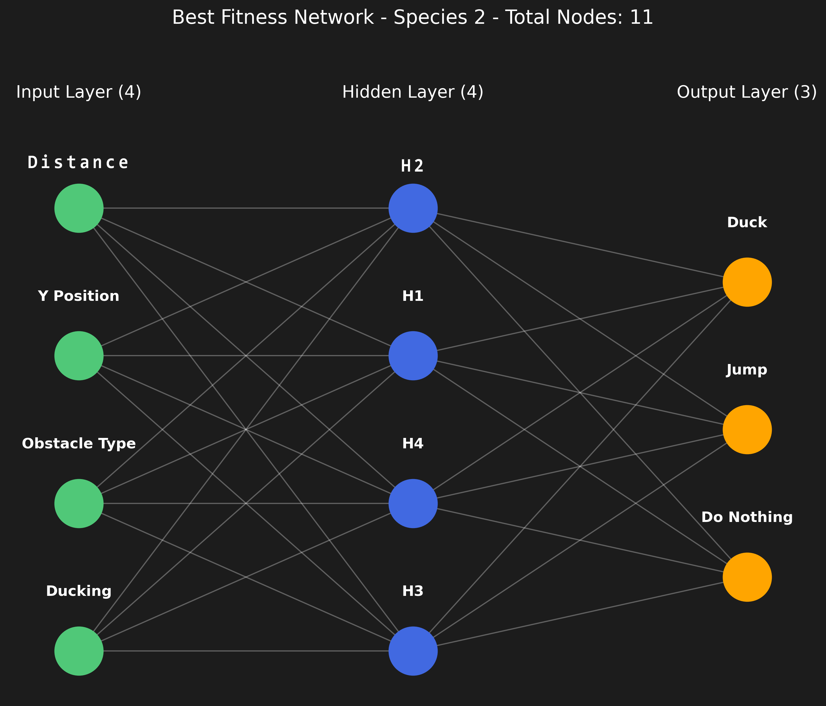
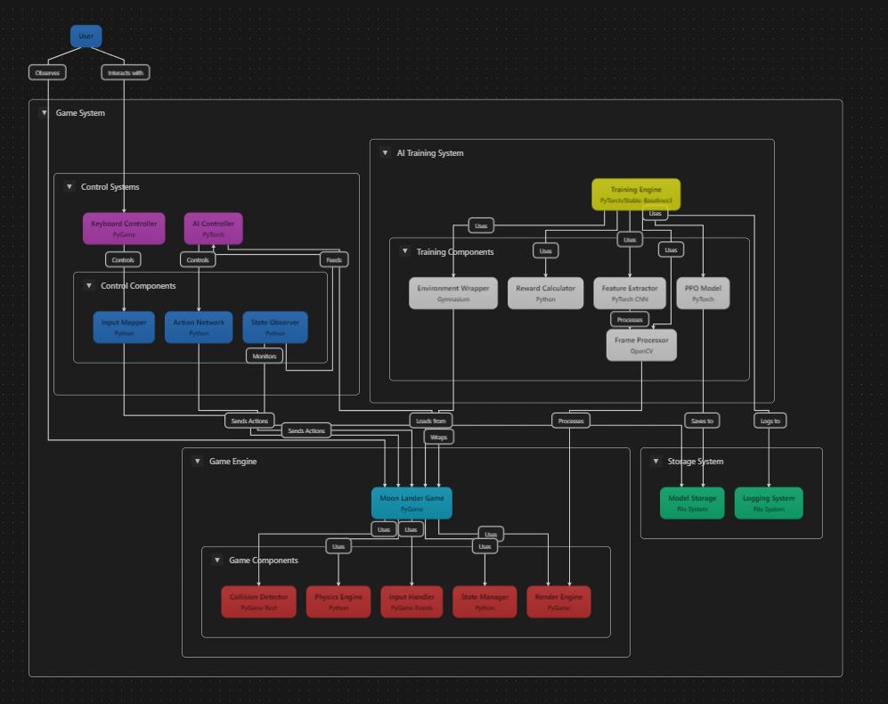
As you can see, using the NEAT algorithm and a large number of members in each population, it managed to build a neural network really quickly to overcome the obstacles in its path. But tuning the settings of NEAT is just the first part. The fun part comes in when you have to decide what NEAT knows about the game world you want it to control. It took me a while to understand that NEAT, and any other RL models, are blind and only rely on what you give it, and it can only do what you allow it. For this first try, I simply gave it 4 inputs: player position, the state of the game character, distance to the next obstacle, and the type of obstacle. It then had to decide 3 things: do nothing, jump, or duck. As mentioned, “do nothing” could have been left out, but this is an exercise in learning, so there you go. Lastly, one had to decide how to reward or punish NEAT. For this first attempt at building something that can learn, I decided to simply reward it for the distance any character traveled and punish it for hitting an obstacle. Below is a much more detailed overview of the input, output, and rewards of NEAT.
Neural Network Inputs:
The network receives the following four input values each frame:
- Player Vertical Position (
player['y']):
This value represents how high or low the player is on the screen. The player starts at ground level and can jump up or stay on the ground. Larger values (near the bottom of the screen) indicate the player is low, while smaller values (if it has jumped) indicate the player is higher above the ground. - Player Ducking State (
int(player['ducking'])):
This is a binary input.1indicates the player is currently in a ducking posture (reduced height).0indicates the player is not ducking.
Knowing whether the player is currently ducking can help the network decide if it should continue ducking, jump, or stand up straight for upcoming obstacles.
- Distance to the Next Obstacle (
distance):
This indicates how far away the next incoming obstacle is horizontally. A larger value means the obstacle is still far off, while a smaller (but positive) value means the obstacle is getting close. As the obstacle moves towards the player, the network should use this information to time jumps or ducks. - Obstacle Type (
obstacle_type_input):
This value differentiates between obstacle varieties:1indicates the next obstacle is a “low” obstacle (located near the ground).0indicates the next obstacle is a “high” obstacle, meaning the player might need to duck rather than jump.
This helps the player’s network choose the correct avoidance behavior (jump over a low obstacle or duck under a high one).
Neural Network Outputs:
The network outputs three values every frame. The code uses output.index(max(output)) to select the action corresponding to the highest-valued output neuron. Thus, only one action is chosen each frame:
- Action 0: Do Nothing
If the first output neuron is the maximum, the player maintains its current stance. If it’s on the ground and not ducking, it remains standing still; if it’s ducking, it continues to duck if instructed. - Action 1: Jump
If the second output neuron has the highest activation and the player is currently on the ground, the player attempts to jump (velocity set upwards). This is key for avoiding low obstacles. - Action 2: Duck
If the third output neuron is the highest and the player is on the ground, the player will duck. This is critical for avoiding high obstacles.
Reward Structure (Fitness):
The script uses a fitness measure to guide the NEAT evolution. The main fitness adjustments occur as follows:
- Incremental Reward per Frame Survived (
ge[x].fitness += 0.1):
Each frame that a player survives (i.e., is still alive and not collided with an obstacle), its corresponding genome’s fitness is increased by 0.1. This encourages networks that keep the player alive longer. - Penalty for Collision (
ge[x].fitness -= 1):
If the player collides with an obstacle, its genome immediately receives a fitness penalty of 1. Colliding results in that player’s removal from the simulation (the agent “dies”). This strongly discourages behaviors that lead to collisions. - Stopping Criterion (
if max_fitness >= 1000):
The simulation for the generation stops if a player reaches a fitness of 1000, indicating that the network has become sufficiently adept at surviving obstacles. Reaching this high fitness value can be seen as a reward threshold for a well-optimized solution.
Now, after having NEAT play and learn for a while and then finally creating a neural network capable of playing my version of the Dino Game, I present to you a representation of the network layout. One would think that something needing to learn even as simple a task as jumping or ducking would require a more complex structure, but no. Initial networks did not have a hidden layer and yet still performed okay. A simple network with only one hidden layer, or even one consisting of just four nodes, managed to play the Dino game perfectly, as you’ve seen in the video.
If you want to run this on your own computer and stare at the wonder of little blocks fighting for their little virtual lives, you can. Below is the link to the GitHub repo with all the code you need to run the same experiment at home. Just don’t start naming the little blocks, please.


NEAT Rocket Version One
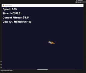
Right, so having figured out the basics of the NEAT algorithm, I decided to give NEAT a slightly harder challenge. How about a rocket that needs to land on a platform? Easy, right? Well, if you know what you’re doing, then sure. However, I wouldn’t count myself among those just yet, at least not at this point. But one needs to start somewhere, and the first step is to build something that the AI can use to train on. So, I had to create a very basic game of a rocket that needs to land on a platform. Naturally, I needed to test the game to see if it’s actually playable. Below is me showing off my skills at not crashing a little rocket. I’m waiting for my NASA invitation, but I’m sure it’s still in the mail.
Now that I had a working game to give to NEAT, I had to build the inputs, outputs, rewards, and penalties again. Not to mention configuring the NEAT config file. So, you can imagine I had a couple of iterations before getting anywhere. I’m not showing this here, but I actually started off with a much more complex game where the platform would move around, and the rocket not only needed to land but also land upright and at a specific speed. That turned out to be a bit too challenging for NEAT to start with, so I decided to train it bit by bit. I decided to give it a simple goal and then slowly start adding more and more complexity to the game as NEAT got “smarter.” I started by placing the rocket in a static starting point on the left of the screen, keeping the platform static, and removing all other game mechanics, just to see if the rocket would learn to fly towards the platform. I did, however, leave in the part where NEAT would be penalized if it did not land the rocket on the platform. Another penalty I had to add was to “kill” any rockets that just hovered up and down without moving in the X direction at all, since I gave each member a specific time to reach the platform. Those that just bounced up and down took up valuable training time and were thus killed very quickly.
Inputs to the System
Action Input:
- Each call to
step(action)receives anactiontuple(rotate_left, rotate_right, thrust).rotate_left(boolean): IfTrue, the rocket’s angle is increased byROTATION_SPEED.rotate_right(boolean): IfTrue, the rocket’s angle is decreased byROTATION_SPEED.thrust(boolean): IfTrue, upward thrust is applied in the direction the rocket is facing.
State Representation (Environment to Neural Network):
The environment’s get_state() method returns a list of 7 normalized values:
self.position.x / self.WIDTHself.position.y / self.HEIGHTself.velocity.x / self.MAX_SPEEDself.velocity.y / self.MAX_SPEEDself.angle / 360(distance.x / self.WIDTH)wheredistance.xis the horizontal distance from the rocket to the platform center(distance.y / self.HEIGHT)wheredistance.yis the vertical distance from the rocket to the platform center
Initial State:
Obtained from reset() which calls get_state(). The rocket’s initial position and platform position are randomized (within specified screen regions), so the initial state varies but follows the same structure above.
Outputs of the System
From step() method:
step(action) returns (state, reward, done, {}) where:
state: The new state after applying the action, structured as described above.reward: A numerical value (float) representing the immediate reward for the chosen action.done: A boolean indicating whether the episode (game) has ended (Trueifgame_overor a terminal condition is met).{}: An empty dictionary (no additional info provided).
Reward Structure and Penalties
The reward is accumulated each step based on events and conditions within the environment:
- Base Reward Initialization:
Each step starts withreward = 0, unless a game-over condition is immediately detected, in which case the reward might be set to -100 at that moment. - Distance-based Reward:
- The code calculates
delta_distance = previous_distance - current_distanceeach step, ifprevious_distanceis known. - If the rocket moves closer to the platform (
current_distance < previous_distance),delta_distanceis positive and thus adds a positive increment to the reward. - If the rocket moves away from the platform,
delta_distanceis negative, thus decreasing the reward.
- The code calculates
- Landing Reward:
- If the rocket successfully lands on the platform (collides with the platform rectangle) with
abs(self.angle) < MAX_LANDING_ANGLEand velocity less thanMAX_LANDING_SPEED, the rocket receives a+1000reward and is reset to a new starting position.
- If the rocket successfully lands on the platform (collides with the platform rectangle) with
- Crashing Penalties:
Several conditions cause the game to end with a penalty of-100:- If the rocket goes out of screen bounds (touches a wall or the top/bottom edges).
- If it touches the platform with too great an angle or too high a speed.
- If the rocket remains at too low speed (
< LOW_SPEED_THRESHOLD) for longer thanMAX_LOW_SPEED_DURATIONwithout landing. - If the rocket stops moving horizontally for longer than
MAX_LOW_SPEED_DURATION.
In all these cases,
game_over = Trueandreward = -100.
Note: Every step’s final reward is added to current_fitness. The current_fitness keeps a running total of the agent’s performance over its episode.
Hyperparameters (Environment Constants)
These are constants defined in the MoonLanderGame class. They govern physics, dimensions, and time scaling:
- Physics:
GRAVITY = 0.1(applied each step downward)THRUST = 0.2(applied when thrust isTrue, in the direction of the rocket’s orientation)ROTATION_SPEED = 3degrees per step (for rotate left/right)MAX_SPEED = 5(velocity is clamped so it never exceeds this speed)
- Landing Conditions:
MAX_LANDING_ANGLE = 360degrees (the code checks ifabs(angle) < MAX_LANDING_ANGLEfor a safe landing)MAX_LANDING_SPEED = 10(velocity must be less than this for a safe landing)
- Low Speed / No Movement Time Limits:
LOW_SPEED_THRESHOLD = 0.9(speed below this for too long triggers a crash)MAX_LOW_SPEED_DURATION = 5000ms (if rocket stays belowLOW_SPEED_THRESHOLDor stationary horizontally for longer than this duration, it’s considered a failure and ends with a -100 penalty)
- Time and Rendering:
CLOCK_SPEED = 400(pygame clock tick rate)TIME_SCALE = self.CLOCK_SPEED / 60(used for time calculations displayed on screen)
Below is the recording of the “left only” training session. I made the number of members in each population about 200 to give it a good chance of at least one or two finding some good path to the platform that later generations could take advantage of. However, it seems that even in generation 0, about 3 of the 200 members managed to build a neural network that was able to land the rocket on the platform. “Landing” is used very lightly here, as you can see from the video. The large spikes on the graph in the game show the members of the population that managed to land on the platform over and over, resulting in a large reward for that specific member.
On a side note, I naturally ran these training steps multiple times, and one would sometimes see very interesting behavior emerging. For example, the rocket below somehow decided to perform a mating dance of the yellow spotted jumping spider instead of landing on the platform. There were many of these strange examples; however, this was the only one I managed to record. Since each network starts from a random state, I was also unable to reproduce any of the other strange behaviors I’ve seen in the many hours of staring at the rocket trying to land.
Well, it seems that NEAT can indeed create a network capable of guiding a rocket from point A to point B, specifically the platform. While I could spend time hardcoding a solution, the appeal lies in leveraging AI for this task. Moving on to a slightly more challenging scenario, I utilized what NEAT learned in the initial phase and made the game more difficult by randomizing the X-axis spawning location. This means the rocket now begins its journey from a random position along the X-axis in the game.
And as you can see from the video, NEAT learned to “land” (crash) the rocket on the platform relatively quickly. Given that it had prior knowledge, this progress was expected. If you look more closely at the video, I started the new game at generation 95, so the neural networks had evolved a bit before starting this new challenge. It still took a while to get to this point, even with its prior knowledge, but I think it’s still very impressive.
Next, I again upped the stakes a bit and changed the spawning location of the rocket to anywhere on the screen. I did add a bit of code to make it not spawn on the platform, as that would be cheating.
And that, ladies and gentlemen, is where the preferred rocket did NOT hit the platform. I tried many different approaches. From starting the training job from scratch to having the rocket resume training where it left off. I even tried splitting the training into multiple windows, each with a dedicated CPU to see if I could speed up training. All for nothing! NEAT just couldn’t get the rocket to land on the platform (well, crash). I tried playing with the hyperparameters, population count, and game speed, but nothing worked. GPT and even Claude were “stumped,” either suggesting things I had already tried or going on a hallucination spree that wasted my time.
NEAT Rocket Version Two
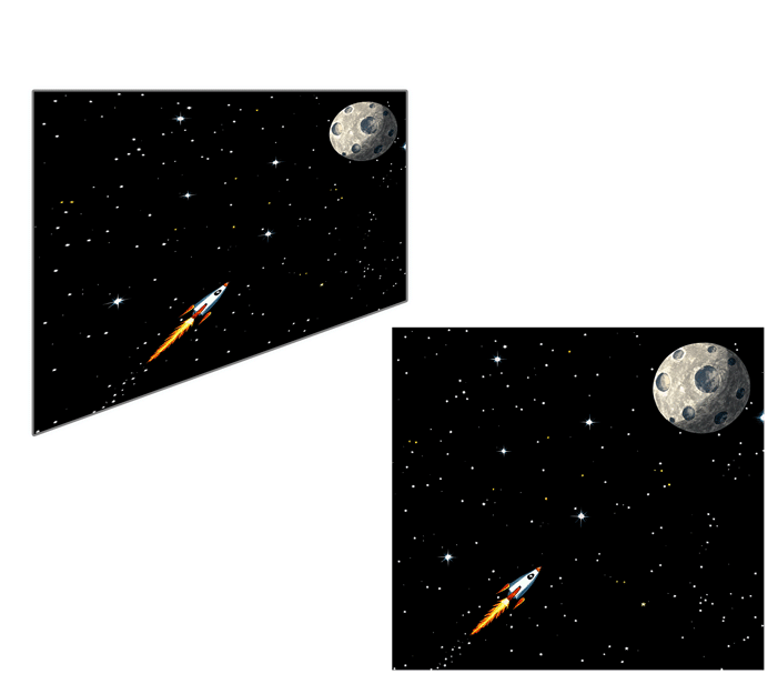
So what do you do? Give up, start over, change the playing field, or play the lottery? Well, yes, I tried all of that. However, the most interesting step for this blog would be to tell you that I started from scratch. Well, not 100%, but I did change the gameplay a bit. This time, instead of having the rocket land on a platform, I altered the game mechanics so that the rocket would need to “chase” the moon. In basic terms, the rocket must fly to where the moon is in the game space. Then, as soon as it reaches the moon, the moon will jump to a random position again. Simple enough, right? Well, yes, for a human! Not so much for an AI not even close to taking over the world. Anyway, I recreated a whole new game from scratch and, of course, I had to test it out. Take note for later: below is me playing the game, NOT the AI.
Once I played a couple of rounds to confirm the game mechanics were sound, and not just to have an excuse to play some games, I handed the controls over to NEAT. I used the basic inputs and outputs similar to the first version of the rocket game. Funny enough, NEAT again had a very hard time training any neural network to even fly the rocket to any location. There were some “signs of intelligence” here and there, but that was equivalent to a drunk guineafowl begging for food. (Yes, we have a few of them around the house, so I know). Even after leaving NEAT to train overnight for about 12 hours straight, at this point, I thought this was where my adventure and claim to fame were going to end. Until I had another look at the inputs the NEAT algorithm was receiving. If you look at the first version, it only had access to seven inputs. Now, I don’t know about you, but if you only were given a stick while being blindfolded, without any other input like sound or even touch, you would have a very hard time navigating anything. And this is basically what NEAT/the rocket had access to to try and learn to fly the rocket. It was basically blind. Poor thing.

So I decided to add additional inputs that NEAT could use to learn and navigate the game environment. The inputs went from 7 to 15. You can see all the additional inputs below.
1. Inputs
The neural network receives the following inputs:
- Horizontal Position: The x-coordinate of the rocket, normalized by the screen width (
self.position.x / self.WIDTH). Range: 0 to 1. - Vertical Position: The y-coordinate of the rocket, normalized by the screen height (
self.position.y / self.HEIGHT). Range: 0 to 1. - Orientation Angle: The rocket’s current orientation angle, normalized by 360 degrees (
self.angle / 360). Range: 0 to 1. - Horizontal Velocity: The x-component of the rocket’s velocity, normalized by the maximum speed (
self.velocity.x / self.MAX_SPEED). Range: -1 to 1. - Vertical Velocity: The y-component of the rocket’s velocity, normalized by the maximum speed (
self.velocity.y / self.MAX_SPEED). Range: -1 to 1. - Normalized Distance to Target: The Euclidean distance to the target, normalized by the diagonal of the screen (
self.position.distance_to(self.target_pos) / math.sqrt(self.WIDTH**2 + self.HEIGHT**2)). Range: 0 to 1. - X Distance to Target: The x-axis distance to the target, normalized by the screen width (
x_distance). Range: -1 to 1. - Y Distance to Target: The y-axis distance to the target, normalized by the screen height (
y_distance). Range: -1 to 1. - Normalized Angle to Target: The angle between the rocket and the target, normalized to the range -1 to 1 (
normalized_angle). - Normalized Angular Velocity: The rocket’s angular velocity, normalized by the maximum angular velocity (
normalized_angular_velocity). Range: -1 to 1. - Relative Horizontal Velocity: The rocket’s x-velocity relative to the stationary target (
relative_velocity_x). Range: -1 to 1. - Relative Vertical Velocity: The rocket’s y-velocity relative to the stationary target (
relative_velocity_y). Range: -1 to 1. - Normalized Distance to Vertical Edge: The distance to the closest vertical screen edge, normalized by the screen width (
distance_to_vertical_edge). Range: 0 to 1. - Normalized Distance to Horizontal Edge: The distance to the closest horizontal screen edge, normalized by the screen height (
distance_to_horizontal_edge). Range: 0 to 1. - Angle Between Direction and Velocity: The angle between the rocket’s direction and velocity vector (
angle_between_direction_velocity).
2. Outputs
The neural network produces three outputs, which control the rocket’s behavior:
- Rotate Clockwise: A value greater than 0.5 triggers a clockwise rotation of the rocket.
- Rotate Counterclockwise: A value greater than 0.5 triggers a counterclockwise rotation of the rocket.
- Thrust: A value greater than 0.5 activates the rocket’s thrusters.
3. Rewards
Rewards are granted to encourage desired behaviors:
- Reaching the Target: The rocket gains 500 points for successfully colliding with the moon (target).
- Distance Fitness: Fitness is calculated based on the reduction in distance from the rocket’s starting position to the target, normalized by the initial distance.
- Increased Time Efficiency: Reaching the target quickly indirectly improves fitness, as prolonged inactivity can result in penalties.
4. Penalties
Penalties are imposed to discourage undesirable behaviors:
- Zero Speed Penalty: If the rocket’s speed is zero for more than 800 milliseconds, 100 points are deducted, and the game ends.
- Zero X Movement Penalty: If the rocket’s horizontal velocity is zero for more than 800 milliseconds, 100 points are deducted, and the game ends.
- Bouncing Off Screen Edges: Collisions with screen edges invert velocity, indirectly reducing performance due to inefficient movement.
After making the changes to what NEAT could see, things started looking much better. Below is the first couple of minutes of NEAT just starting out the training process with the newly updated inputs. I did keep the part of the code that “killed” off any member of the population that had the rocket just fly up and down with no left or right, as those never recovered and just wasted training time. It was really interesting to see each neural network try something else at the start of the training. Some did spins, others just got stuck in the corners, while others seemed to literally hit their head against the side of the window for some reason.
Below is a video of NEAT finally making progress. Not great, but still making progress, it seems to get the concept that it should navigate towards the moon; however, when it got close, it just hovered there. Perhaps it was assuming the moon would come to it. Like a teen at his first prom, not knowing how to approach the girl he has a crush on.
And finally, after many, many hours of training, NEAT finally managed to get a couple of networks to reliably fly the rocket to the moon, and then redirect it to wherever the moon might appear next. Note that I’m saying reliably, meaning it can do it every time. I did not say it did it well! It seems it has learned it in a couple of steps: step one, move the rocket to the same Y-axis as the moon; step two, do a very awkward side shuffle in the direction of the moon. Rinse and repeat. Well, it got the job done, I guess. This half reminds me of the reinforcement learning algorithms that were tasked with training a human-like creature to walk and run. It did so in the end, but it looked like it did not understand the basics of its own body.
Well, as you can see from the video below, NEAT did not disappoint. I’m sure that if I let NEAT train for even longer, it would eventually find an even better way to reach the moon. Or I just needed to play more with the rewards and penalties for this version. However, this was good enough for me.
I saved some data from each population and graphed the fitness of each one. As you can see, it took a really long time for NEAT to make any progress. And it’s only in the last couple of generations where a member of the population got lucky and produced a combination of neurons that was able to play the rocket game sufficiently.
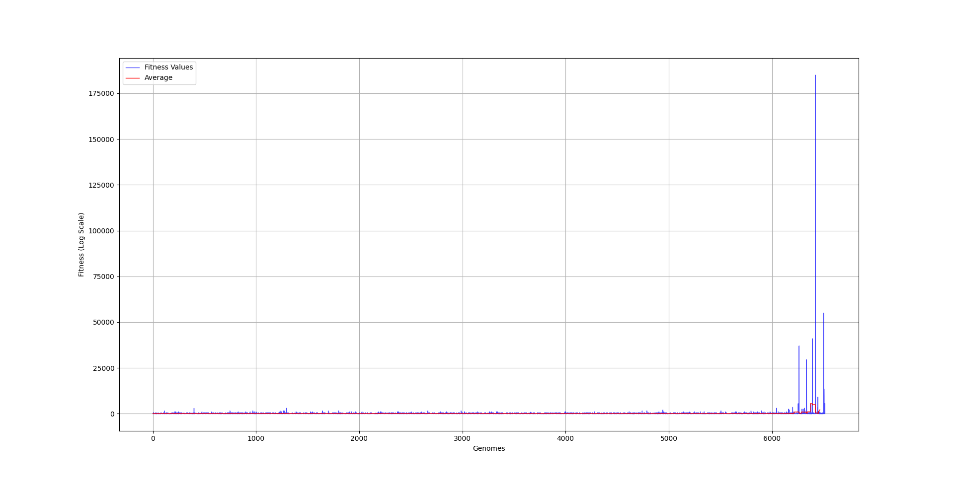
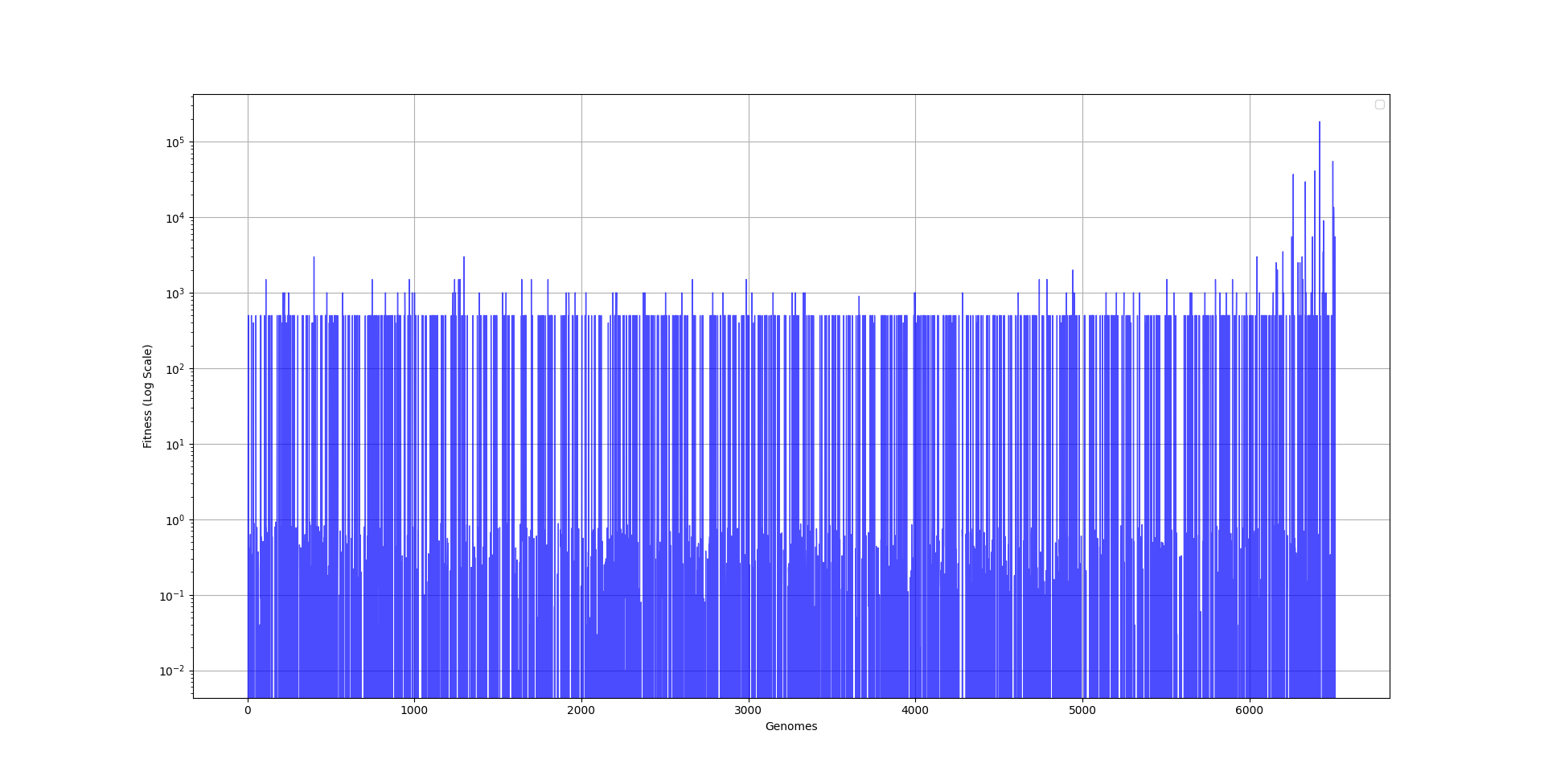
Since the last couple of generations managed to do so much better than all those before, the graph is a little bit hard to grasp, so I created a logarithmic version of it, showing that most populations did not manage to procure anything that was really worth evolving upon. I guess that is how life also works. It can take billions of years for the first cell to figure out how to move towards getting more energy, and it only took the human race a couple of hundred years to go from “candle and chill” to “oh look, the AI can do my job better than me”.
I was interested to see how the neural network of the best model actually looked. I was rather surprised that it was still rather simple. Then again, it only needed to fly a rocket in 2D space from point A to point B, but still, it was rather impressive for such a simple network.

Moving on to even bigger and better ways of doing things, in the beginning of this article, I mentioned two types of reinforcement learning approaches I wanted to explore: NEAT being the first, and now on to the Actor-Critic type of architecture.

Actor-critic is a powerful approach to reinforcement learning that elegantly divides the learning process between an “actor,” which chooses actions, and a “critic,” which evaluates how good those actions are. Imagine an experienced driving instructor (the critic) teaching a young learner (the actor) how to drive. As the learner navigates the roads, the instructor provides feedback—highlighting mistakes (like drifting out of lane) and applauding successes (smooth turns or safe braking). This guidance helps the learner distinguish which driving habits to keep and which ones to change. In the same way, the critic estimates how beneficial each action might be, and the actor adjusts its choices based on that evaluation.
Over time, the learner-driver picks up better habits and the instructor’s critique becomes more precise. The instructor refines the way feedback is given, while the learner steadily internalizes these lessons, making fewer mistakes on the road. This mirrors the actor-critic loop: the actor’s policy (its decision-making process) improves as it receives clearer assessments from the critic, and the critic becomes ever more accurate as it observes how the actor behaves. Thanks to this harmonious interplay, the actor-critic method offers both efficient learning (through guidance from the critic) and the freedom for the actor to experiment with new strategies, ultimately leading to increasingly sophisticated decision-making.
Difference between DDPG, SAC and PPO
Actor Critic is the a sub section of reinforcement learning, however within this there are also a couple of method one can approach the Actor Critic way of reinforcement learning. Here is a quick break down of the methods I tested.
Proximal Policy Optimization (PPO), Soft Actor-Critic (SAC), and Deep Deterministic Policy Gradient (DDPG) are popular methods for training agents in continuous control tasks, but they approach the problem in different ways. DDPG focuses on learning a deterministic mapping from states directly to the best action it can find. In other words, once trained, the policy simply outputs a single action each time without any built-in randomness. While this directness can be powerful, DDPG often requires careful tuning and thoughtful exploration strategies, as its deterministic nature makes it harder to adapt if the environment is complex or if the agent needs consistent, varied exploration.
SAC, on the other hand, always keeps a dose of randomness in its actions. Rather than going all-in on what looks like the best action so far, it encourages the agent to stay curious by deliberately maintaining some uncertainty. This built-in exploration tends to produce more stable training, making SAC easier to get good results with minimal tinkering. By balancing the pursuit of high rewards with maintaining a “broad” policy that doesn’t get stuck on one strategy, SAC usually adapts well to a variety of tasks, even those where it’s not immediately clear what the best actions might be.
PPO also uses a stochastic policy, but it has a different priority: it tries to refine the policy without making drastic jumps. PPO relies on fresh data from the current version of the policy (making it on-policy), and it introduces a “clipping” trick to avoid taking overly large, potentially harmful steps. This careful approach helps keep training stable and predictable. Although PPO may need more frequent data collection—since it doesn’t reuse old experiences as efficiently as SAC or DDPG—its reliability and ease of implementation have made it a popular choice in many research and practical scenarios. In short, DDPG can be powerful but finicky, SAC is more robust and exploratory, and PPO strikes a comfortable balance between steady improvements and practical simplicity.
PPO
First I decided to give PPO a try instead of the NEAT algorithm. Here is bit deeper dive into what makes PPO such a useful algorithm to use.
Proximal Policy Optimization (PPO) is a popular reinforcement learning algorithm that elegantly combines concepts from both value-based and policy-based methods. It is built around the notion of maintaining a good balance between improving the agent’s policy and ensuring these improvements remain stable and reliable.
Key Concepts Behind PPO:
- Actor-Critic Architecture:
At its core, PPO uses an actor-critic framework. The actor is a neural network that outputs a probability distribution over possible actions given a state—this represents the agent’s policy. The critic is another neural network that estimates the value of states or state-action pairs. By learning these two functions simultaneously, PPO can leverage the critic’s value estimates to guide and stabilize the training of the actor. - Policy Gradients and Unstable Updates:
Traditional policy gradient methods adjust the actor’s parameters directly in the direction that increases the likelihood of good actions. While this can be effective, it can also lead to unstable learning. A single large update can push the policy too far, causing it to diverge or worsen rather than improve. - Clipped Objectives and Proximal Updates:
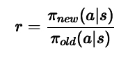
PPO introduces a special “clipped” objective function to prevent overly large policy updates. Instead of allowing the new policy to stray too far from the old policy at each training step, PPO constrains the update so that the ratio of new to old action probabilities stays within a specified range.Concretely, if the old policy said the probability of taking action A in a certain state wasπ_old(a|s), and the new policy suggestsπ_new(a|s), PPO looks at their ratio:If this ratio deviates too much from 1 (beyond a certain threshold, often 20%), PPO “clips” the objective to stop encouraging changes that are too large. This ensures updates are proximal, meaning they don’t drastically move the policy away from what it was previously doing. By keeping these steps small yet effective, PPO achieves more stable learning. - Advantage Estimation (GAE):
To determine how good or bad an action was compared to what the agent expected, PPO uses advantage functions. The advantage tells you how much better (or worse) it is to have chosen a particular action over the baseline expectation.A refined method known as Generalized Advantage Estimation (GAE) is often used. GAE reduces the variance in advantage estimates, producing more stable and reliable learning signals. With these more stable advantages, PPO can update the actor to favor actions that genuinely yield higher long-term returns rather than just short-term gains or lucky outcomes. - Mini-batch Optimization and Multiple Epochs:
PPO also adopts a flexible training loop. After the agent collects a batch of experience—states, actions, and rewards—it performs multiple epochs of stochastic gradient descent on that batch. Instead of discarding the batch after a single pass (as some other policy gradient methods do), PPO reuses it a few times. This increases sample efficiency and ensures that the policy is thoroughly improved with the information currently on hand before moving on. - Balancing Exploration and Exploitation: PPO includes entropy regularization in its objective function. Adding an entropy term encourages the policy to maintain some level of randomness, which helps prevent premature convergence to a suboptimal policy. By not becoming too deterministic too quickly, the agent can continue exploring different actions that might lead to better solutions.
Why PPO is Popular:
- Stability: The clipped objective keeps updates conservative and prevents large, destabilizing changes.
- Simplicity: While PPO improves upon older methods like TRPO (Trust Region Policy Optimization), it is conceptually simpler and often easier to implement.
- Efficiency: PPO strikes a good balance between sample efficiency (making good use of the data it collects) and reliable convergence, making it suitable for a wide range of tasks—from robotics simulations to complex video games.
In Short:
PPO refines policy gradient updates by clipping them, ensuring the new policy remains close to the old one and thus maintaining stable learning dynamics. By combining value-based guidance (through the critic), advantage estimation, and controlled policy updates, PPO reliably improves the policy over time without the wild oscillations or catastrophic failures sometimes seen in other methods. This careful approach to updating the actor’s behavior has made PPO a go-to method for both researchers and practitioners in reinforcement learning.
I redid the inputs, output, rewards and penalties a bit for PPO after playing around more with all the parameters as well.
INPUTS OUTPUTS REWARDS PENALTIES
State Inputs (Observations)
At each step, the agent receives the following normalized inputs as its observation state:
- Horizontal distance to target (x_distance):
(target_pos.x - rocket_pos.x) / WIDTH
This measures how far the rocket’s x-position is from the target’s x-position, normalized by the screen width. - Vertical distance to target (y_distance):
(target_pos.y - rocket_pos.y) / HEIGHT
Similar to the horizontal distance, but now for the y-axis, normalized by the screen height. - Relative angle needed to face the target (normalized_angle):
First, the angle to the moon (angle_to_moon) is computed usingatan2. Then, the difference between the rocket’s current angle and angle_to_moon is calculated and normalized to the range [-180, 180], and then divided by 180.
This tells the agent how far off its orientation is from directly facing the moon. - Normalized X velocity (normalized_velocity_x):
(velocity.x) / MAX_SPEED
The horizontal component of the rocket’s velocity, normalized by a maximum speed constant. - Normalized Y velocity (normalized_velocity_y):
(velocity.y) / MAX_SPEED
The vertical component of the rocket’s velocity, also normalized by MAX_SPEED. - Normalized angular velocity (normalized_angular_velocity):
(current_angular_velocity) / MAX_ANGULAR_VELOCITY
The rate of change of the rocket’s angle (degrees per second), normalized by a maximum allowed angular velocity. - Distance to vertical edge (distance_to_vertical_edge):
min(position.x, WIDTH - position.x) / WIDTH
How close the rocket is to the left or right boundary of the screen, normalized by the width. - Distance to horizontal edge (distance_to_horizontal_edge):
min(position.y, HEIGHT - position.y) / HEIGHT
How close the rocket is to the top or bottom boundary of the screen, normalized by the height.
These 8 values form the observation vector provided to the agent at each step.
Actions (Outputs)
The action space is a 3-dimensional continuous vector (each dimension from -1 to 1), which are then discretized into specific rocket control actions. For the sake of clarity:
- Action input: A 3D vector
[a0, a1, a2]where each component is in [-1, 1]. - Action interpretation (converted to discrete control):
The environment interprets these continuous actions into seven binary “switches” that represent different levels of rotation and thrust:- Strong right rotation if
a0 > 0.5 - Weak right rotation if
0.1 < a0 <= 0.5 - Strong left rotation if
a1 > 0.5 - Weak left rotation if
0.1 < a1 <= 0.5 - Strong thrust if
a2 > 0.7 - Medium thrust if
0.3 < a2 <= 0.7 - Weak thrust if
0 < a2 <= 0.3
If these conditions are not met, the corresponding control is not applied. The agent effectively decides how to rotate left or right and how much thrust to apply.
- Strong right rotation if
Rewards and Penalties
The reward function is composed of multiple components that encourage the agent to move closer to the moon, point in the correct direction, and reach the target efficiently, while penalizing actions that don’t help or that lead to stagnation.
Reward Components:
- Distance improvement reward/penalty:
- Let
prev_distancebe the rocket’s distance to the target before the step, andcurrent_distancebe the distance after the step. - Distance Improvement:
(prev_distance - current_distance) * 5
If the rocket gets closer to the target (distance decreases), it earns a positive reward. The larger the improvement, the bigger the reward. - Distance Worsening: If the rocket moves away from the moon (
current_distance > prev_distance), an additional penalty of(distance_improvement * 10)is added. Sincedistance_improvementis negative in this case, this results in a negative reward. This strongly discourages moving away from the target.
- Let
- Angle alignment reward:
- The code calculates
relative_angleto the moon’s position. A perfect alignment grants a positive reward, and facing away yields a penalty. - The scaling chosen is
(180 - relative_angle) / 18.0, which yields values from about -10 to +10. Facing the moon can give up to +10 reward, while facing away can give up to -10.
- The code calculates
- Thrust direction penalty:
- If the rocket is thrusting while facing away from the moon (
relative_angle > 90degrees), it gets a -5 penalty. This discourages wasting thrust when not oriented towards the target.
- If the rocket is thrusting while facing away from the moon (
- Constant time penalty:
- A small penalty of
-0.1per timestep is applied to encourage the rocket to reach the target quickly rather than loitering indefinitely.
- A small penalty of
- Path efficiency penalty:
- A penalty based on how long it’s taking the rocket to reach the target compared to a straight path. This is calculated as:
efficiency_penalty = -0.01 * (steps - (straight_line_distance / MAX_SPEED))
The penalty is capped at a maximum of -1 per step. This discourages overly roundabout paths.
- A penalty based on how long it’s taking the rocket to reach the target compared to a straight path. This is calculated as:
- Target landing reward:
- If the rocket collides with (hits) the target moon, it receives a large reward bonus:
Base hit reward:+1000
Time bonus: An additional bonus that starts at2000and decreases by2each step is added. For example, hitting the target quickly yields a high time bonus, while taking longer reduces it. The total upon hitting the moon can easily surpass+2000if done quickly.
- If the rocket collides with (hits) the target moon, it receives a large reward bonus:
- Stationary penalty:
- If the rocket’s speed remains too low (
velocity.length() < 0.1) for too long (more than5 * CLOCK_SPEEDframes), the episode ends and the rocket receives a large penalty of-100. This prevents the agent from simply standing still and doing nothing.
- If the rocket’s speed remains too low (
Episode Termination Conditions
- The agent can quit if the game window is closed (returns a terminal state).
- The agent can become “stuck” and get a stationary penalty, terminating the episode.
- The agent may continue indefinitely until total training steps are reached (in practice, training code handles termination).
Summary
- Inputs: Rocket-to-target distances (x, y), angle error, velocities, angular velocity, and distances to edges of the screen.
- Outputs: Continuous actions converted into discrete rotation and thrust levels.
- Rewards: Primarily driven by getting closer to the target, aligning with the target, efficient path-taking, hitting the moon for large rewards, and moderate time penalties.
- Penalties: Given for moving away from the target, thrusting in the wrong direction, idling too long, and inefficient paths.
Environment Dynamics and Constants
- Screen dimensions:
800 x 600 - Gravity :
0.05 - Thrust :
0.5 - Rotation speed :
3degrees per step - Maximum speed :
3 - Clock speed :
60FPS (Sets how often the environment updates per second)
Below is a list of the main hyperparameters used in the provided training code and environment. These parameters influence both the training process (through PPO and vectorized environments) and the environment dynamics.
PPO (Stable-Baselines3) Hyperparameters
- Policy:
MlpPolicy
Uses a multilayer perceptron (a fully connected neural network) as the underlying policy and value function approximator. This means the policy and value functions are both represented by neural networks with several fully connected layers. - Learning rate:
5e-4(0.0005)
Controls how quickly the neural network parameters are updated. A higher rate can speed up learning but risks instability, while a lower rate provides more stable learning but can slow convergence. - Number of rollout steps (n_steps):
2048
Defines how many steps of the environment the agent runs before performing a gradient update. Larger values mean the agent collects more data per update, which can improve stability at the cost of using more memory and longer iteration times. - Batch size:
256
The number of samples the algorithm uses in each minibatch when updating the policy. The batch size influences how stable the gradient updates are. Larger batches can provide smoother updates, while smaller batches increase update frequency and responsiveness. - Number of epochs (n_epochs):
10
Each batch of collected experience is reused for multiple passes (epochs) of gradient updates. More epochs mean more thorough training on the same data, potentially improving sample efficiency but increasing computation time. - Discount factor (gamma):
0.99
Determines how much the algorithm discounts future rewards. A value close to 1.0 means the agent considers long-term rewards almost as important as immediate ones, while a lower value emphasizes more immediate rewards. - GAE lambda (gae_lambda):
0.95
Used in Generalized Advantage Estimation (GAE) to reduce variance in policy gradients. A value closer to 1.0 considers advantage estimates over more steps, while a smaller value relies on shorter horizons. - Clip range (clip_range):
0.2
The PPO objective “clips” the policy updates to avoid overly large updates in a single training step. This parameter sets how far new action probabilities can deviate from old probabilities before being penalized. - Entropy coefficient (ent_coef):
0.01
Encourages exploration by rewarding policy entropy. A higher value means the agent is penalized less for being uncertain (i.e., having a more spread-out probability distribution over actions), promoting more exploration. - Policy network architecture (net_arch):
Specifies the size and structure of the neural network layers.- Policy network layers (pi):
[512, 512, 512, 512, 512, 512, 512, 512, 512, 512]
This defines ten consecutive layers each with 512 neurons for the policy network. A very large network capable of representing highly complex policies, but also computationally expensive. - Value network layers (vf):
[512, 512, 512, 512, 512, 512, 512, 512, 512, 512]
Similar architecture for the value function network, helping it accurately predict the value of states. The large capacity aims to learn a detailed value function representation.
- Policy network layers (pi):
Environment & Training Setup Hyperparameters
- Number of parallel environments (num_envs):
10
Used withSubprocVecEnvto run multiple instances of the environment in parallel. - Total training timesteps:
10,000,000 - Checkpoint frequency (save_freq):
10,000steps
The model is saved as a checkpoint at every 10,000 training steps. - Reward logging frequency (check_freq):
1,000steps
Rewards are logged at a frequency of every 1,000 steps per environment. - Monitor Wrapper: Used around each environment instance to track and log episodes.
For interest sake here is a visual of the code running and training the rocket:
So now it was time to start the training session. Well, I started the training session multiple times while getting all the parameters right, however, below is the final version that seems to learn very quickly. As mentioned before, the nice thing about PPO is that you can again have multiple versions of the game running at the same time, but this time, all the experiences built up are being fed into a single network instead of each game having its own network like NEAT. This also meant that the training time was significantly less than NEAT. Where I had to leave NEAT training for almost a day, PPO managed to get a working rocket going in about an hour!
Below is a recording of PPO starting its training session. I had 10 games running at the same time, but I only had enough screen space to show two at the same time.
And now, for those who are interested, below is the full training session. This was the first hour, and I stopped the training shortly after this as the rocket managed to get to the moon every time! This is sped up about 4X. You will see there is a pause every now and then. This is where the critic is updating the actor network on how the training is going. Then, once this is completed, the game continues. So, in this case, the updating of the actor network is not real-time, but every X number of steps. I think in this case, it was every 1000 steps or so.
Below is a graph I created from the stats I saved during the training session. You will see in the video that the fitness for every game goes into the negative before slowly getting back to zero. Then, as the PPO algorithm learns, the rewards for each game add up. Each game is slightly different, as there is still some manner of randomness built into PPO. But just by looking at this graph, you can see how quickly PPO learns to control the rocket vs NEAT.
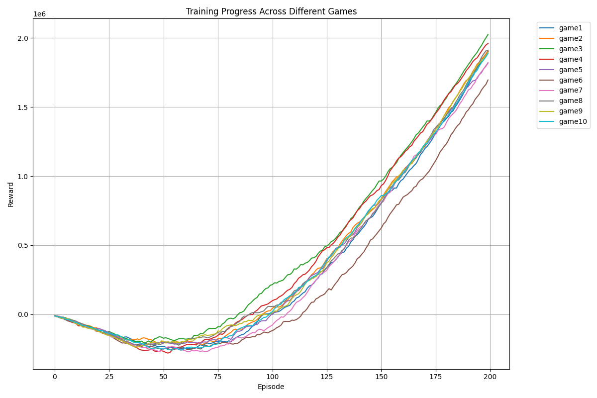
And now for the final results. This is the best model saved as a separate model so one can replay this anytime you want. You can see there is a huge difference in gameplay compared to NEAT. Although to be fair, the penalties, inputs, and rewards for NEAT were not as well thought out as PPO, but still.
If you would like to play with all the code for the project yourself you can find it in my GitHub repo below. Any comments would be welcome.
Soft Actor-Critic (SAC)
Next, I wanted to see how SAC compared to PPO. Using the baseline3 library, it was rather easy to switch the code from PPO to SAC with only changes to a couple of lines of code. All the inputs, outputs, rewards, and penalties were kept the same. I was very pleasantly surprised to see that SAC trained even faster than PPO; the version I came up with had no need for the critic to update the actor every X number of steps, and this happened every step in the background without any slowdown in training time. For the moment, SAC will be my go-to reinforcement learning algorithm for the rest of this project.
As you can see below, SAC managed to train much quicker, resulting in fewer episodes needed and hardly ever going negative in terms of the number of rewards accumulated.
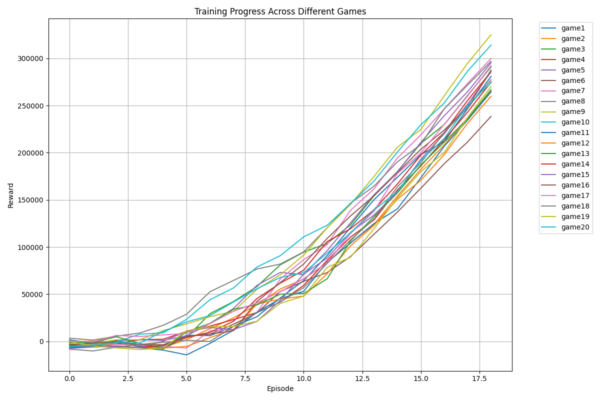
Below is the sped-up version of the full training session. The entire training session only took about 20 minutes before I stopped it. And if you ask me, SAC gave the most “human-like” gameplay if you compared it to when I played the game manually myself. Again, keep in mind that the window you see below is only one of the 20 games being played at the same time.
DDPG
Earlier, I mentioned that I also played with DDPG. And yes, I did experiment with DDPG a lot; however, I would say that this one was a bit of a failure. Or, rather, I did not know how to implement it decently. The main obstacle I ran into was the noise that is added to the actor network. With DDPG, the noise “level” is decreased every step, eventually leaving both networks to rely only on exploitation and not exploration. This means that the networks then only use what they have learned and do not try anything new anymore. I played a lot with the noise level, and how quickly the noise should be reduced, etc.; however, every time the network fell short of learning a decent model before the noise level became too low. Like I said, I’m sure this is a PEBKAC issue and not the fault of the DDPG architecture; however, I’m sure SAC would still beat DDPG, and thus this is the network I’m going to use for further experiments.
Rocket Vision

Right after the successful test models I created so far, I figured I might as well see how far I can take things. What if, instead of the model getting numerical inputs to train on, it was given a photo of the actual game? So, instead of things like the X, Y coordinates, speed, velocity, etc., all it was able to see was an image of the game itself, like a human. Easy, right? I mean, use something like OpenCV to capture the game window, extract a screenshot of the game. Then downscale the game into something that the AI can work with, say a 100×100 pixel image. Then take that image and convert the RGB values to a 3 x 100 x 100 numpy array, with each cell containing the RGB values for that specific pixel. Then give that to the AI to figure out what to do to make the rocket fly towards the moon. I mean, in theory, that would make sense, right? I mean, that’s how they train cars to drive autonomously, right? Below is an account of my attempt at doing just that. Well, spoiler alert, there is a reason why the people who do this for a living get paid so much.
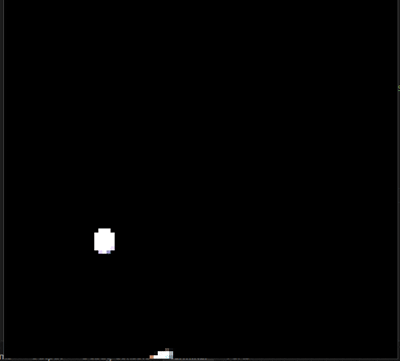
Above is a screen recording of my first attempt. I basically did what I described above. The small window on the top left is the game window. The bigger pixelated one next to it is the captured image scaled down to 100×100 pixels. And the big window on the right is a representation of the numpy array containing the values for each pixel, separated by red, green, and blue. I know it’s a bit small to read, but each value is printed there, and I made the text color the same as the color being represented, because why not. So far, so good. On to my first training session.
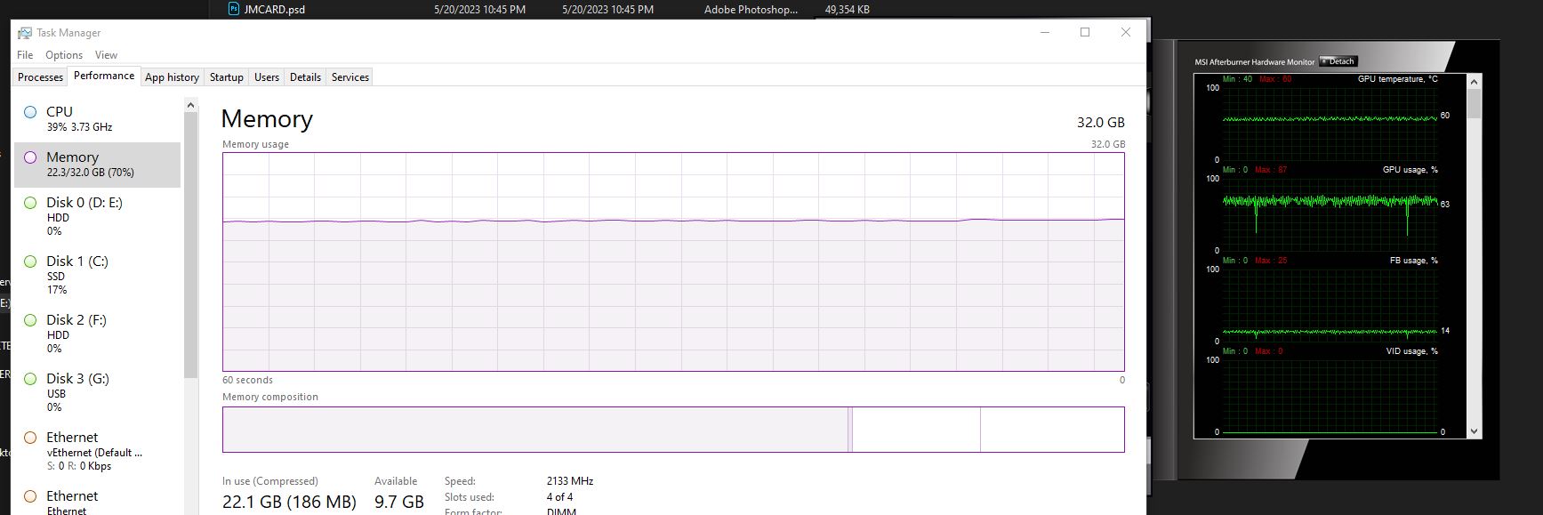
It turns out that having images as input instead of a couple of parameters does seem to tax your computer a bit. 300,000 input parameter inputs needed a neural network that was able to handle and process all of this. I found this out via trial and error. It seems that having a 2-layer x 256 network did not really cut it. And this is not even speaking of the batch sizes and the history buffer. And trying to get everything into memory was a bit of a mission. I have 32GB of RAM, and the training crashed so many times I stopped counting. Also, playing with things like the batch size to make use of the CPU and the VRAM was also a game of tweak the dials and see what breaks. On one hand, the training did not crash, but either the CPU or GPU was sitting idle for most of the time. And if I changed things too much, either my PC would crash, and once I even got a blue screen of death when my GPU ran out of VRAM and the program just exited stage left. I did, however, get some training to actually train for a while, but even after about 24 hours or more, there did not seem to be any improvement in how well the rocket was able to fly towards the moon.
Time for another approach: frame stacking. I initially thought I was sooooooo clever coming up with the idea of giving the AI multiple frames to train on. Seems other, much smarter people thought of this long before it came to me. The idea behind frame stacking is that if you look at a single image, you cannot see where the rocket is going since it’s just a snapshot in time. However, if you show a human or AI alike a couple of frames of something, you can then determine a lot more things like speed, direction, acceleration, etc. So, what you do is you take a couple of screenshots of the last four frames of the game and feed that to the AI. My version, which I had before realizing this was already thought of, was to take the 4 screenshots and build a single new frame with all the 4 snapshots layered on top of each other with some transparency added. The older the frame, the higher the transparency. The idea was that, since the transparency was different, the RGB values in each cell of the numpy array would also be different, thus giving the AI something to work with to determine what the rocket was doing prior to the last frame.
Above is my version of frame stacking with me playing the game. (I with the AI could do this!) I mean, it looks very cool, but yes, it was not very practical in the end. Or, I just did not know how to make full use of this as a decent input for the AI to train on. In this whole exercise, I fully blame myself for this experiment not working, and I’m sure others would have made this work in a couple of hours or less. Turns out that the common way of doing frame stacking was to just feed the 4 frames separately to the AI and not build a new frame with all the images squashed on top of each other. Sure, in the end, the 3x100x100 gets converted to a 3x300x100 array, which then gets flattened to a 30,000-element array for the AI to process the data better. And yes, I did also have a look at the 30,000-element array to make sure all the frames were there.

After many training attempts, I decided to make it even easier on the AI. I also realized, after the fact, that this was also a common way of working with images. Simply convert the color image into black and white. This way, instead of having 3 channels, you now only have 1, ranging from 0-255. I thought this might help speed up the training, as each “successful” training, aka, not crashing, ran for many, many hours. Above is a screenshot of one of those attempts, with multiple games running. The windows you see are a visualization of the numpy array, where each pixel is showing the number in that cell. And yes, I did spend way too long just looking at these stupid little rockets buzzing around the screen like mindless idiots.
Above is one such mindless idiot suffering from a massive case of social anxiety. Perhaps I should have made it green instead of black and white, then it would have looked like some night vision version of the game.
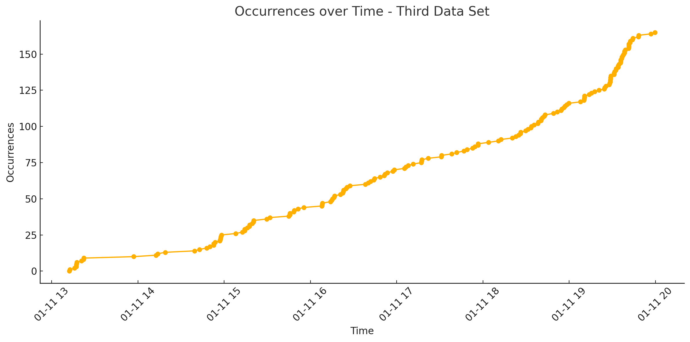
Well, after another day or so of training, there was not much progress. Well, there were some. The rockets went from just flopping on the ground to flying randomly (this accounted for 90% of what you see above) to then again hiding in the top corners of the game window with full throttle. I tried so many combinations of changing the rewards and penalties; I stopped after putting in rewards or penalties I’ve already tried in the past. The graph above seems like there is progress, especially at the end, but this was after about running the training for almost a week non-stop. My GPU was not happy with me, and I think if I’ve done this in the winter, it would actually have been a good thing, as my office was really hot with the GPU making everything so nice and toasty. Sorry, back to the graph, as I said, it seems like there is progress, but remember this is 150 hits in a WEEK, so I would not really call that progress. What you want to see is nothing in the beginning and then, after a while, an exponential spike in hits as the AI starts to learn what is going on. Okay, sure, it’s also needed to learn basic physics based on 4 images, so you know I have to give it some credit for doing anything.
![]()
I then decided to make things even easier for the AI. I scaled down the 100×100 image to 64×64 pixels. Oh, and I rewrote the entire game from scratch, this time with everything just being blocks. Above is a representation of what I came up with to feed the AI. The image in the middle is a text-based representation of the numpy array, just to make sure what is in the array is actually what is going on in the game. I also moved away from a 0-256 index to just 3: nothing, moon, player. That is it. On the left is a matplotlib graph showing the numpy array in a visual form, and on the right is the actual game. Ohhhh… just look at those ray-traced specular reflections.

Keep in mind that above is the actual size of the game, but since I don’t like putting my nose against my screen more than I have to, I scaled up all the windows a bit to see what is going on. This is a 64×64 pixel game I call “Pixel Lander”. I’m just waiting for EA Games to contract me for the deal.
In the theme of taking things very slowly, I only now started adding any functions dealing with rewards or penalties. Keep in mind, no AI anywhere, yet. The video above shows the game window along with a graph of the rewards of the game in real-time. Basically, the closer the rocket gets to the moon, the more rewards it gets for every step or frame of the game. You will see a small bump when the rocket hits the moon; this is intended as a little carrot with icing on top for getting to the moon. The large spike in the graph was me not playing the game while setting up the screen recording; I built in a huge penalty for the rocket not moving at all. The window on the right is the 4 frames used for frame stacking. See, that little explanation earlier now comes in handy, hey? You will see each frame is a little bit behind the other. I also graphed this to make sure this is the case, as in the beginning, I just had the same frame duplicated multiple times, and rotated 90 degrees for some reason.
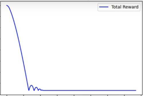
Something interesting to see in the first second or two of the video is the little graph before it went off a cliff. This was me starting the game; the rocket spawned in the middle of the screen and fell down to the bottom of the screen, doing a little bounce before becoming stationary. This would then correlate to the distance the rocket was from the moon, hence getting fewer rewards, except for the little bounce where it was again slightly closer to the moon. I’m glad the physics of the game is working as it should.
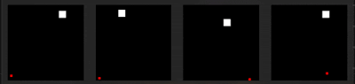
Well… after all that effort and trying almost every combination of training parameters, the result above is the best I could manage. In most cases, the rocket either fell to the ground or just flew up to the top of the screen… you know, screw trying to get to the moon or anything. Sigh… Oh well… Time to cry and say:
Yes… I spent so much training time on this part of the project, not to mention all the time spent on building and fine-tuning the model. I even sometimes used cloud computing to throw just raw power at the problem, but no such luck. Well, I must say it was not for nothing. Insert quote about Edison, who tried 1000 versions of how not to make a lightbulb. I also learned a lot more about reinforcement learning in the process, and I will use all I have learned for my next projects, so it definitely was not all for nothing. So, I’m still going out with a smile on my face, albeit with a couple of bumps and bruises.
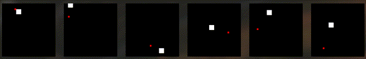
So, just to give myself a little bit of a boost in motivation, I opted again to train the same game using more traditional training methods. In other words, not giving the AI an image, but the raw input parameters. This time, I only gave the model basic inputs, such as the X and Y locations of the rocket and the moon. I again used the SAC RL model to train this, and guess how long it took to train the AI to play this massively complicated game? About one and a half minutes. I retrained it a couple of times, just because I was used to training times taking hours, if not days, to get this result, which never happened.

Below is the graph showing every time the rocket managed to hit the moon during training. You can see that in the beginning, it was sparse, and then after about a minute, it managed to understand what needed to be done, and off it went. Looking at the blue graph above, you can see that it settles very quickly into an almost 45-degree line, where it has reached peak performance and is now only limited by the physics of the game.
